3.3 How does PERMANOVA do it?

Following the PERMANOVA table of results, a suite of key additional details regarding the analysis can be seen in the PERMANOVA output file. These details highlight what makes the implementation of PERMANOVA in PRIMER so unique, surpassing all other software tools that we know of in its handling of multi-factorial sampling and experimental designs.

The implementation of PERMANOVA in PRIMER pays very careful attention to whether factors are fixed or random and whether they are crossed with or nested within other factors in the study design. The construction of correct test-statistics and permutation algorithms for every term in the model rely ciritically on the expectations of the mean squares.

Additional details in the PERMANOVA output file include (Fig. 3):

• details of the expected mean squares (EMS) for each term in the model;
• the construction of the pseudo-F ratios for each term in the model from the appropriate mean squares (along with the associated numerator and denominator degrees of freedom); and
• estimates of the components of variation for each term in the model in the space of the resemblance measure.

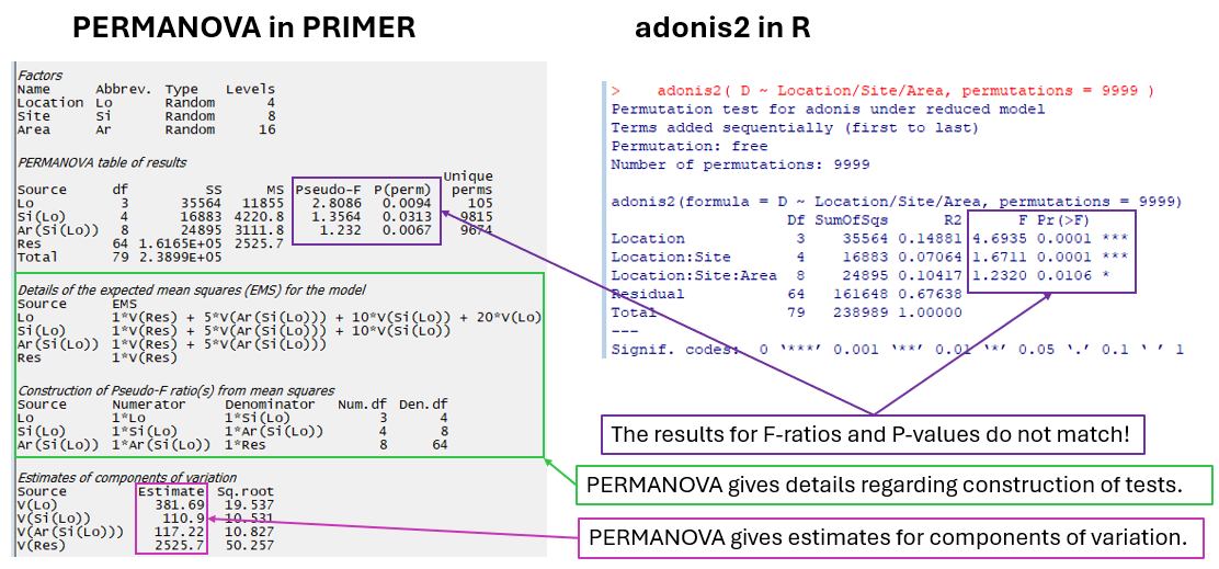Fig. 3. Additional details provided in the output from a PERMANOVA analysis.

Expectations of mean squares

This portion of the output file shows which components of variation are involved (may contribute towards) the expectation of any given mean square (MS). For example, consider the mean square for the factor 'Location'. It is clear from the above output that variation among replicate holdfasts ('V(Res)'), Areas ('V(Ar(Si(Lo)))'), Sites ('V(Si(Lo))') and Locations ('V(Lo)') are all involved and hence can potentially contribute towards the expectation of the mean square (EMS) for Location.

Why do we bother with this? When we test individual terms in our model, it is absolutely vital that we build an F-ratio that focuses only on testing the null hypothesis associated with the term of interest. We must make sure not to confound its source of variation with other potential sources of variation inherent in our experimental design when we perform each individual test.

Construction of pseudo-F ratios

PERMANOVA in PRIMER uses the EMS information in order to contruct the correct pseudo-F ratio for the test of any individual component of variation (term) in any multi-factor model. This is done with careful consideration of fixed and random factors in mixed models and/or hierarchical (nested)-type study designs. For example, it is appropriate, in this three-factor nested study design, to construct the individual tests as follows:

Source	Construction of pseudo-F statistic
Location	$F$$Lo$ = $MS$$Lo$ / $MS$$Si(Lo)$
Site	$F$$Si(Lo)$ = $MS$$Si(Lo)$ / $MS$$Ar(Si(Lo))$
Area	$F$$Ar(Si(Lo))$ = $MS$$Ar(Si(Lo))$ / $MS$$Res$

It would be incorrect, of course, to test 'Location' by placing $MS$_$Lo$ directly over the residual mean square ($MS$_$Res$) as the denominator. That approach will not account correctly for the other sources of variation (Areas and Sites) that may indeed contribute towards the mean square for 'Location'. This is true for multivariate dissimilarity-based analysis, just as it is for classical univariate ANOVA.

Permutable units

The denominator of the pseudo-F ratio also points us directly towards the correct permutable units for the test ( Anderson (2001b) ; Anderson & ter Braak (2003) ). By 'permutable units', we mean the items that should be considered 'exchangeable' under a true null hypothesis. Hence, if we are interested in testing the factor of 'Location', we must permute whole sites (there are 8 of them, and we need to keep the replicates within each site together as a unit) randomly across the 4 locations. It is not appropriate to permute replicate holdfasts just anywhere randomly across the entire study design for the test of 'Locations', just as it is not appropriate to use the residual mean square directly as the denominator for the test of 'Locations'.

The implementation of PERMANOVA in PRIMER always uses expected mean squares to get a correct rigorous test for every term in the model; specifically:

• to construct the correct pseudo-F ratio; and
• to implement a correct permutation algorithm, accounting for other terms in the model.

Permutation algorithm

P-values are obtained by PERMANOVA in PRIMER using permutation algorithms that are constructed specifically for each term in the model, after identifying:

• the correct permutable units (referencing the F-statistic's construction); and
• the correct reduced-model residuals, accounting for other terms in the model.

Using reduced-model residuals is the default in PERMANOVA. Alternatively, one can choose to permute raw data or full-model residuals, which are less optimal, but are fine asymptotically. Even so, this does not get away from the need to ascertain the correct permutable units, which is not really negotiable if you want to achieve the correct test for your study design.

Of course, each term will require its own denominator and its own permutation algorithm, which will depend on whether terms are fixed or random, whether there are nested terms, covariates or interactions, etc. For unbalanced cases, the 'Type' of sum of squares is also very important for the partitioning, the expectations, and subsequent tests.

Degrees of freedom

The additional information provided in the output also helps us to see where the degrees of freedom (df) from our full study design 'ended up' in the PERMANOVA analysis. From an experimental design point of view, it is important to try to maximise the denominator df, whenever possible, in order to obtain better power for tests of the term(s) of interest. For example, if we wanted to get more power to test for significant variability at the scale of Locations, then increasing the number of holdfasts per area would do little to help. We would be far better off increasing the number of sites sampled per location (even at the expense of reducing the number of holdfasts collected per area), precisely because the mean square for 'Site' is used as the denominator in the pseudo-F statistic constructed by PERMANOVA to test for variation among Locations.

Components of variation

Finally, the estimated components of variation are also extremely useful (provided at the bottom of the output file). These are calculated in a directly analogous way to univariate ANOVA estimators, relying (once again) on the expectations of the mean squares. The column labeled 'Estimate' is in squared dissimilarity units, and its square root ('Sq.root', interpretable as a sort of standard deviation in the space of the resemblance measure) is also provided.

In the present example, we can see that the greatest variation occurs at the smallest spatial scale - from holdfast to holdfast within a given area (i.e., the square root of 'V(Res)' is 50.257 in Jaccard % dissimilarity units). This means that holdfasts that are just a 'fin-kick' away (or so) from one another may share little more than half of their mollusc species! The sources of variation (in order of importance, as quantified by the PERMANOVA model) are: Residual > Location > Area > Site.

The values in the 'Estimate' column can be expressed (optionally) as percentages of the total (provided there are no negative estimates of variation in a given model), thusly:

Source	Estimate (based on EMS)	Percentage
Location	381.69	12.17 %
Site	110.90	3.54 %
Area	117.22	3.74 %
Residual	2525.70	80.55 %
Total	3135.51	100.00 %

It is not uncommon in ecological field studies for the residual component of variation to be large relative to other sources of variation.

For more information about all of these key additional details provided in the PERMANOVA output file, please consult the PERMANOVA+ manual.