An analysis of biotic data
Rationale
Multivariate data are very complex and can be difficult to analyse and interpret. Each variable can be considered its own dimension, with its own story to tell. Thus, when there are a lot of variables (e.g., if we have sampled occurrence, abundance, or biomass of individual species in a community, and each species is a variable), then we have a very high-dimensional system to consider. We can choose to analyse each variable individually, but this would be time-consuming if we have a lot of variables. Also, for biotic data, many species are rare, so our data will be riddled with a large number of zeros - it would be difficult to characterise anything about individual rare species on their own. Furthermore, what we are usually aiming to do is to characterise and analyse the whole community simultaneously and how it may be changing through time or space, or in response to some experimental treatments (such as human impacts or management scenarios, etc.).
When analysing multivariate biotic data (especially those having a large number of variables), a useful approach is to base the analysis on a resemblance measure (i.e., a dissimilarity or similarity measure), calculated among the sampling units (e.g., Clarke (1993) , Anderson (2001a) , McArdle & Anderson (2001) ). A resemblance measure such as Bray-Curtis captures the ecological idea of turnover in the identities and relative abundances of species beween any pair of sampling units ( Clarke et al. (2006) , Anderson et al. (2011) ). For many routines in PRIMER, the fundamental starting point is a resemblance matrix, which expresses (numerically) the (dis)similarities between every pair of samples.
Before calculating a resemblance matrix, some pre-treatment of the data (sometimes in more than one way) is usually desirable. For assemblage data, an overall transformation can be used to reduce the dominant contribution of abundant species towards Bray-Curtis similarities. For example, a fourth-root transformation will down-weight the influence of highly-abundant taxa.
From a resemblance matrix, we may readily apply the following methods (Fig. 5.1):
- Cluster analysis, to help characterise inter-sample relationships, showing potential groups of similar samples;
- Ordination, to help visualise inter-sample relationships in a small number of dimensions (usually 2 or 3); and
- Hypothesis-testing, to formally test a particular null hypothesis of interest, such as H0: 'There are no differences in community structure among different (a priori) groups of samples'.
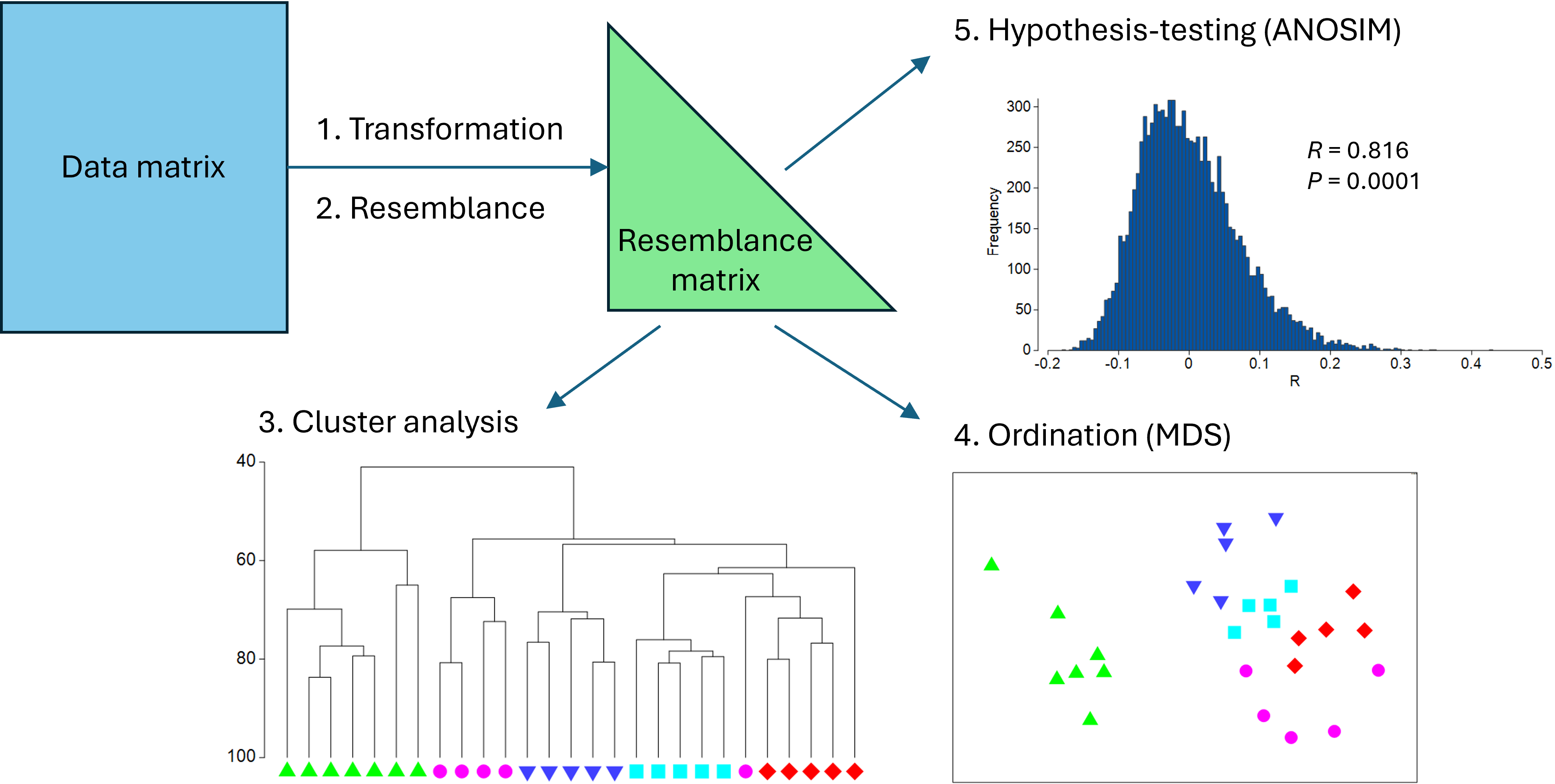
Fig. 5.1. Schematic diagram of a simple multivariate analysis pathway, including transformation, resemblance, clustering, ordination and hypothesis-testing.
Some steps for analysis
In what follows, we shall take the 'Fal nematode.pri' example dataset in PRIMER and proceed along a simple multivariate analysis pathway according to the following steps:
- Apply a fourth-root transformation to the data (all variables).
- Calculate the Bray-Curtis resemblance among all pairs of samples.
- Calculate a hierarchical group-average cluster analysis of the samples to produce a dendrogram.
- Create a non-metric multi-dimensional scaling (nMDS) ordination plot of the samples.
- Use the analysis of similarities (ANOSIM) to test the null hypothesis of no differences in community structure among the 4 creeks of the Fal estuary (with n = 5 to 7 replicates per creek).