Step 5: Ordination of centroids
Having seen the results of a PERMANOVA analysis, it is natural to wish to see a visualisation of the patterns among centroids belonging to different groups or combinations of levels of different factors in the study design. In many cases, particularly if there is a large number of replicates in a complex study design, if one were simply to create an ordination of all individual sampling units, there would just be a lot of noise (the plot may look very messy), due to high residual variation. This tends to obscure salient patterns and important effects.
Ordination of sampling units (all replicates)
We can produce a non-metric MDS ordination of the holdfast data by starting from the Jaccard resemblance matrix and clicking on Analyse > MDS > Non-metric MDS..., taking all of the defaults, then clicking OK. The resulting configurations are very unsatisfactory with quite high stress, either in 2 dimensions (stress = 0.28, shown below), or 3 dimensions (stress = 0.20).
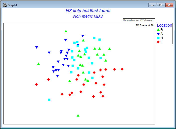
Seeing a bit of a 'mess' when we plot replicates like this is actually not too surprising in many cases, and particularly in this case, considering the very high variation (high turnover) in the identities of molluscs among holdfasts at small spatial scales (within areas), as seen on the previous page (recall that the residuals contributed by far the greatest source of variation to this system).
Ordination of distances among centroids
We can instead examine an ordination plot of the centroids in the space of the resemblance measure. In multi-factor designs when there is more than one factor and these factors are crossed with one another, we may need to created a single factor that consists of combinations of levels of the crossed factors (using Edit > Factors... > Combine...), but in the case of a fully nested design, and where nested factors all utilise unique labels (such as we have here), we can proceed without such a step.
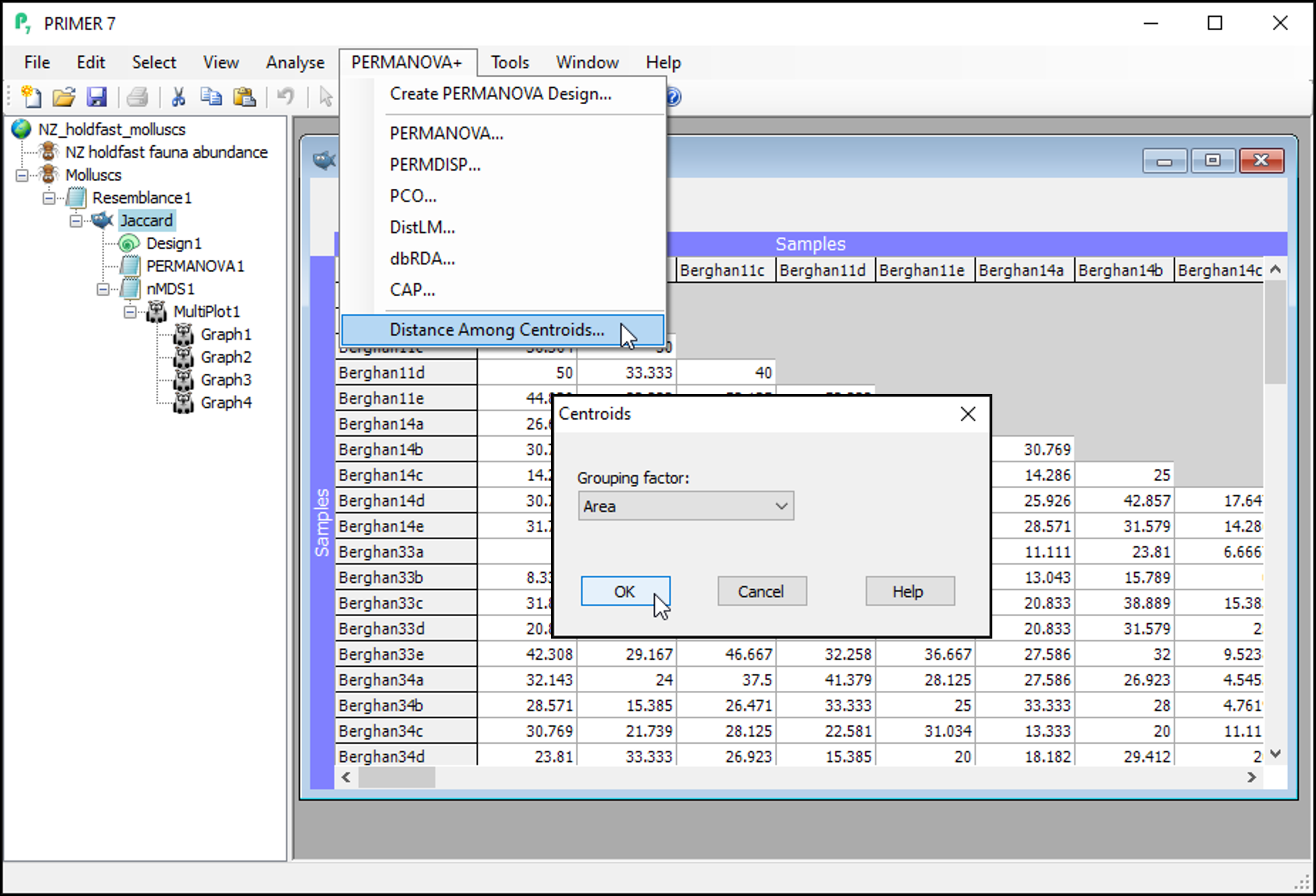
- From the 'Jaccard' resemblance matrix, click PERMANOVA+ > Distances Among Centroids, then in the 'Centroids' dialog, choose (Grouping factor: Area), and click OK.
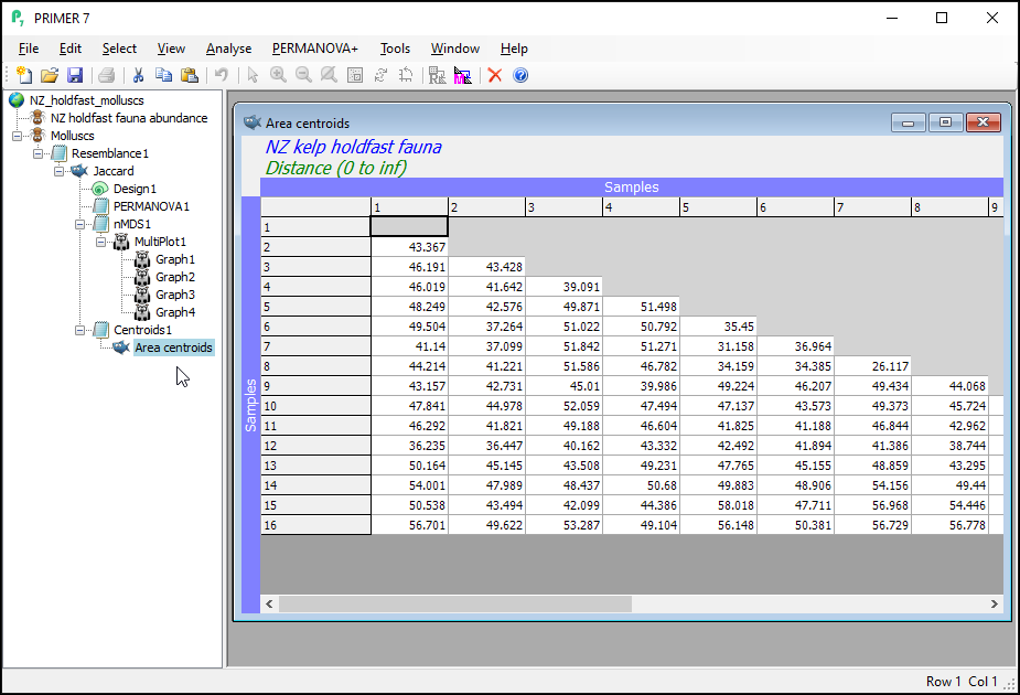
This will give you a matrix of Jaccard dissimilarities among the 16 Area centroids; each centroid being comprised of n = 5 replicate holdfasts within a given area. These are constructed in the space of the dissimilarity measure, which is not (quite) the same thing as calculating the arithmetic averages in the space of the original variables (i.e., that corresponds to a centroid in Euclidean space). In other words, these are the centroids just 'as PERMANOVA sees them' in Jaccard space, when doing the partitioning. You can re-name this matrix (from 'Resem1') to 'Area centroids'; i.e.,
-
From the 'Area centroids' resemblance matrix, click Analyse > MDS > Non-metric MDS..., take all the defaults and click OK.
-
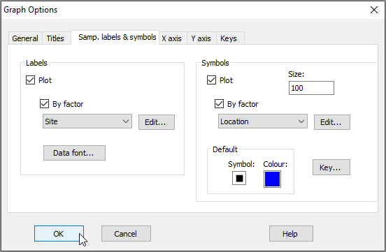
From the 2D nMDS (probably called 'Graph5'), click on Graph > Sample Labels & Symbols..., then choose (Labels > $\checkmark$Plot > $\checkmark$By factor > Site) & (Symbols > $\checkmark$Plot > $\checkmark$By factor > Location), then click OK.
The result is a much more interpretable ordination plot, with far lower stress, viz:
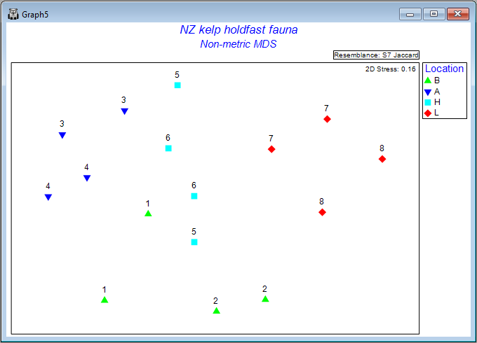
Each point now represents the centroid (in Jaccard space) for n = 5 holdfasts in a given area. The numbers identify the 8 different sites, and the colours correspond to the 4 different locations. The patterns we see here are consistent with what was learned from the PERMANOVA analysis. More specifically, we can see that, within any particular location, the variation from one area to the next (any 2 centroids having the same symbol and number) is fairly similar to the variation between the two sites (any 2 centroids having the same colour, but a different number), and also that variation among locations (different colours) exceeds this - all four locations are clearly distinguishable from one another on the plot.