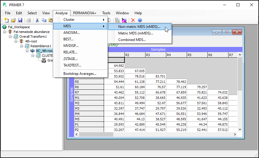
Step 4: Ordination
The cluster analysis goes some way towards helping us to understand potential patterns of similarity among the samples. It is particularly good at showing us clusters of samples that are highly similar. To better visualise patterns of relationships among all of the samples simultaneously, we can use methods of ordination. In particular, non-metric multi-dimensional scaling (nMDS) is a wonderfully robust tool for visualising high-dimensional systems on the basis of a chosen resemblance measure ( Kruskal & Wish (1978) ; Clarke (1993) ). Non-metric MDS essentially places points into an arbitrary Euclidean space of set dimension (typically producing a 2D or 3D plot) so as to preserve, as well as possible, the rank-order of the dissimilarities between pairs of samples. For more details on multi-dimensional scaling, see Chapter 5 of 'Change in Marine Commmunities'.
Create a non-metric MDS plot
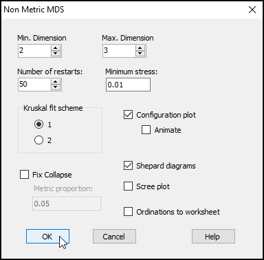
From the Bray-Curtis resemblance matrix ('BC_4th-root' in this example), click Analyse > MDS > Non-metric MDS..., then click OK to run the MDS algorithm with all of the default options.
The resulting 'Multi-plot1' output graphic gives you 4 individual plots (in a 2-by-2 array), as follows:
- the best 2D solution (from 50 random starts)
- the Shepard diagram for the best 2D solution
- the best 3D solution (from 50 random starts); and
- the Shepard diagram for the best 3D solution
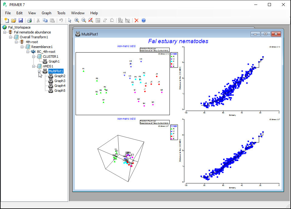
Clicking on the '+' symbol next to the word 'MultiPlot1' in the Explorer tree reveals the four graphics that comprise this multi-plot object ('Graph2', 'Graph3', 'Graph4', 'Graph5'). If you then click on 'Graph2' in the Explorer tree, or if you click in the Multi-plot itself on the plot in the upper left-hand corner, you will see a single graphic now; namely the best (lowest-stress) 2-dimensional non-metric MDS plot for the Fal estuary nematodes.
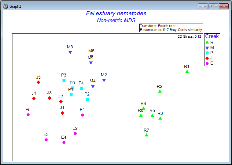
Interpretation
The plot does not have x and y axes, as the scale here is arbitrary. The non-metric MDS algorithm attempts only to preserve rank-order dissimilarities, so interpretations are restricted to relative distances among points in the plot. For example, we can make statements like: "The dissimilarity between sample R7 and M3 appears to be larger than the dissimilarity between sample M3 and M2", but we cannot tell (directly from the plot) what the specific sizes of those particular dissimilarities are.
It is clear from this output that Restronguet Creek ('R') has assemblages of nematodes that are quite dissimilar from those found in the other four creeks. That's consistent with what we saw in the cluster analysis of these data. We can, however, get quite a few more insights from the nMDS plot than were apparent in the cluster dendrogram. For example, relationships among the assemblages from the other four creeks seem to be ordered (from the bottom-left towards the top of the plot) as follows: Percuil → St. Just → Pill → Mylor. It is also apparent that the samples from Pill Creek ('P') form a tighter cluster hence are not as variable as the samples from (say) Restronguet Creek ('R'), which are more spread out. Being able to see potential gradients of change in assemblages, the degree of between-group differences, as well as the relative sizes of within-group dispersions, is all very useful.