12.2 Classical univariate control chart
A classical univariate control chart arises in the context of process control for industrial and other systems. A control chart tracks the value for a particular process variable of interest by plotting a suitable statistical charting criterion versus time, and provides a rigorous test of the null hypothesis that the process remains 'in control' at each individual time-point ( Montgomery (2020) ).
For example, suppose we have a factory that produces spools of thread, and we have a specific machine that churns out individual spools of thread, one after the next. We have a known expected (target) value for the mean diameter of the spool that we wish to produce, by design, which is $\mu$. There is also some level of variation in diameters, $\sigma$, due to some vagaries of the process, that is also known by us a priori.
With the system to produce the spools of thread all set up, we then monitor each consecutive spool being produced by measuring its diameter. Here, our variable is $Y$ = the diameter of the spool of thread, and $\text{E}(Y) = \mu$ and we have $\text{Var}(Y) = \sigma^2$. We measure consecutive values (one for each spool being produced) as $y_1, y_2, y_3, \ldots$. Thus, at any particular time-point $t$, we have observation $y_t$, which is the measured diameter for the spool of thread produced at that time.
Shewhart control chart
A classical Shewhart control chart ( Shewhart (1931) , Shewhart (1939) , Fig. 12.1) plots the values $y_t$ through time, and also includes a horizontal line on the plot to show the expected value $\mu$, as well as two additional horizontal lines corresponding to:
- an upper control-chart limit: UCL = $\mu + 3\sigma$ and
- a lower control-chart limit: LCL = $\mu - 3\sigma$.
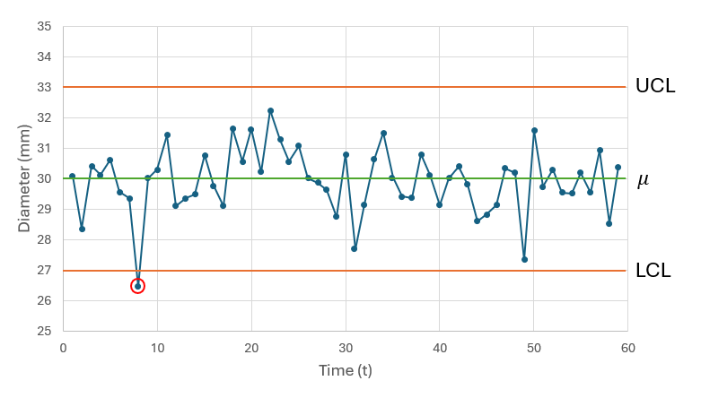
Fig. 12.1 Univariate control chart for the hypothetical example, plotting the measured diameter of spools of thread vs time, with $\mu$ = 30 (green horizontal line) and $\sigma$ = 1. Upper and lower control chart bounds (UCL and LCL, respectively) are shown as orange horizontal lines. Samples that fall beyond the control-chart limits (circled in red) are deemd to be 'out of control'.
The essential idea here is that we want to have proper control over the quality of the spools of thread we produce. We want to identify any cases where the system is, in some way, going 'out of control'. Specifically, any spools of thread that have a diameter falling outside of the acceptable control-chart limits should trigger an alarm of some kind so that some remedial course of action can be taken. For example, in Fig. 12.1, the 8th sample (circled in red) is 'out of control' (falling below the LCL), so that particular spool of thread might be thrown out, as it does not conform to the standard of control we require. The production of an out-of-control sample might also trigger us to stop the system entirely to check for errors in production or machinery that may need to be fixed.
Setting the control-chart limits
The classical UCL and LCL ($\mu \pm 3\sigma$) are set such that values within 3 standard deviations of the expected value are deemed to be 'in control'. In practice, however, assuming the variable is aproximately normally distributed, we can set the 'level-to-reject' ($\alpha$) to whatever we consider appropriate in a given context. Using a multiplier of 3 corresponds to the limits being set at the 0.001 and 0.999 quantiles of a normal distribution, which amounts to $\alpha$ = 0.002 (i.e., 0.1% in either tail). A multiplier of 1.96 would correspond to the limits being set at the 0.025 and 0.975 quantiles (hence $\alpha$ = 0.05 overall, with 2.5% in either tail).
Other univariate control-chart methods
The above is a description of the earliest and most fundamental example of a control chart. There have been a large number of further developments in the general field of statistical process control (SPC) since the early work of Shewhart in the 1930's. For more on this topic, see Barnard (1959) , Quesenberry (2007) and Montgomery (2020) .