7.4 Example: environmental impact on molluscs

The study design

We consider here a study examining effects of a sewage outfall for $p$ = 151 mollusc species from subtidal habitats (3-4 m depth) in the Mediterranean Sea along the southwestern coast of Apulia, Italy ( Terlizzi et al. (2005) ). Abundances of each species were obtained from each of $n$ = 9 replicate 20 cm x 20 cm quadrats in each of three random sites (separated by 80-100 m) at the outfall location ('I', putatively impacted), and at each of two control locations ('C1' and'C2'). Overall, there was therefore a total of $N$ = 81 sampling units: 9 replicates within each of 3 sites within each of 3 locations (Fig.7.3).

Important: the two control locations were chosen randomly from a set of 8 possible such locations along that particular coastline, which were separated by at least 2.5 km and which provided comparable environmental conditions (in terms of slope, wave exposure, type of substratum) to those occurring at the outfall.

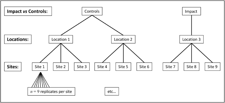
Fig. 7.3 Schematic diagram of the hierarchical design used by Terlizzi et al. (2005) to examine effects of a sewage outfall on subtidal molluscan assemblages.

The ANOVA model for this design has three factors:

• Impact vs Controls ('IvC', fixed with $a$ = 2 levels)
• Locations ('L', nested in IvC, with $b_1$ = 2 controls and $b_2$ = 1 impact location)
• Sites ('S', random and nested in L with $c_{j(i)}$ = 3 for all $j = 1,\ldots,b_i$ and all $i=1,\ldots, a$.

Is the factor of 'Locations' fixed or random? Well, the $b_1$ = 2 control locations were chosen randomly from a finite population, having a total size of $B_1$ = 8 possible control locations. This yields a sampling fraction of $b_1/B_1$ = 1/4 for the controls, whereas there was only one (fixed) impact location, hence $B_2$ = 1 and $b_2/B_2$ = 1. When we set up the design file to run this model to assess the response of the whole assemblage (based on the Bray-Curtis resemblance measure), using the PERMANOVA routine in PRIMER 8, we will be able to specify precisely this design, including details of the finite nature of the population of control locations from which we have sampled.

Note that the onus is on us, as researchers, to specify the size(s) of any finite population(s) of levels for each factor as precisely as we can, as part of our design. This means we have to consider carefully just what the population of levels actually is that we are drawing from for any random factor, and, therefore, the genuine spatial extent of the inferences we intend, and will be able to make, from the analysis. In some cases, particularly at large spatial scales, as in this case, a random factor may be finite. This shifts it, along the sampling-fraction progression, towards being considered more like (though not entirely as) a fixed factor (see Fig. 7.2). Conceptually, it makes sense that if we know more about the population (because we have sampled a greater fraction of its possible levels), then we will accordingly (generally) have more power to draw specific inferences about that population.

Examine patterns in the multivariate data

1. Start running PRIMER 8, then click File > Open... to open the data file named 'Med_molluscs_counts.pri' (found inside the 'Examples_P8 > Med_molluscs' folder).

2. Get the resemblance matrix among the sampling units based on the Bray-Curtis measure. Click Analyse > Resemblance... > (Measure > $\bullet$ Bray-Curtis similarity) & (Analyse between > $\bullet$ Samples). The resulting resemblance matrix will be called 'Resem1'.

Interest lies in examining variation among sites and locations in this hierarchical design. It would therefore be useful to observe an ordination of resemblances among the averages of the 9 sites (based on the identities and relative abundances of mollusc species they contain), and to get a visual sense of the variability in those averages across the locations, rather than viewing a (noisy and high-stress) ordination of relationships among all of the replicate quadrats.^†

We will therefore examine an ordination of bootstrap averages at the scale of Sites for this example. Specifically, within each site, we will bootstrap re-sample (with replacement, in a suitable number^‡ of dimensions, $m$) the $n$ = 9 quadrats a total of $n_{\text{boot}}$ = 50 times. We then calculate fifty corresponding bootstrap averages (1 from each bootstrap re-sample) for each site, and plot these all together in a threshold-metric multi-dimensional scaling ordination based on the Bray-Curtis resemblances among them. We will also choose to output the $m$-dimensional bootstrap averages themselves, just to give us more flexibility for plotting.

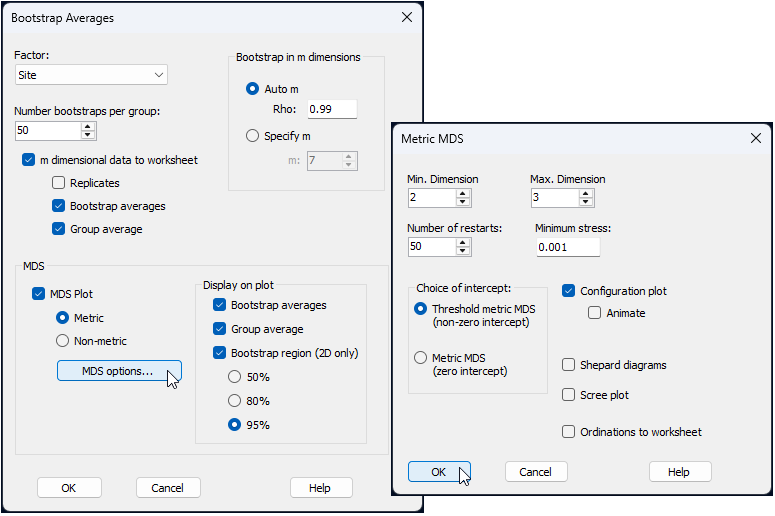
3. From the 'Resem1' similarity matrix, click Analyse > Bootstrap Averages... and choose the following options (leaving the rest as defaults):

   $\hspace{0.5 cm}$> Factor: Site
   $\hspace{0.5 cm}$> Number bootstraps per group: 50
   $\hspace{0.5 cm}$> $\checkmark$ m dimensional data to worksheet
   $\hspace{1.0 cm}$ $\checkmark$ Bootstrap averages
   $\hspace{1.0 cm}$ $\checkmark$ Group average
   $\hspace{0.5 cm}$> $\checkmark$ MDS Plot > $\bullet$ Metric, then click the button that says 'MDS options...' and pick
   $\hspace{1.0 cm}$ Choice of intercept: $\bullet$ Threshold metric MDS (non-zero intercept)
   

all as shown in the dialog windows below:

The default bootstrap average ordination plot (called 'Graph1' in the Explorer tree after you run the bootstrap averaging) can be tweaked by changing the colours, labels, symbols, etc. (just click Graph > Sample Labels & Symbols... and click on the 'Key' button). If you want even finer control, you can work from the $m$-dimensional bootstrap averages themselves, output as 'Data1' here. Specifically, from 'Data1':

• (i) calculate the Euclidean distances among all of these samples (they are the full set of bootstrap averages) by clicking Analyse > Resemblance... > (Measure > $\bullet$ Euclidean distance) & (Analyse between > $\bullet$ Samples).; and
• (ii) create a threshold metric MDS of this Euclidean distance matrix by clicking Analyse > MDS > Metric MDS (mMDS / tmMDS...).

Changing the symbols/labels of the output graphic (which would be output in an item labeled 'Graph3' in the Explorer tree, based on the above steps) essentially gives Fig. 7.4, shown below.

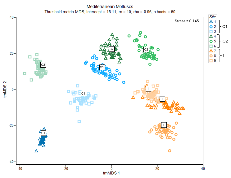
Fig. 7.4 Threshold-metric MDS plot of the averages of three sites from each of three locations in the study design ("C1", "C2" and "I", labeled inside white squares), along with 50 bootstrap averages (coloured symbols specific to each site) for subtidal molluscan assemblages in the Mediterranean, based on Bray-Curtis resemblances.

Average assemblages in sites at the impact location ("I", shown using symbols coloured with orange hues) appear to be quite separate and distinguishable from those occurring at either of the control locations ("C1" in blue hues and "C2" in green hues) (Fig. 7.4). It is not clear, on the face of it, however, whether this difference would be sufficient to be detected as statistically significant, because there is quite a lot of variability among control sites and potentially a difference between the two control locations as well.

Create the design file

To run a PERMANOVA on these data, we first need to create a design file that matches the study design.

4. Make as many rows as there are factors - From the original resemblance matrix ('Resem1'), click PERMANOVA+ > Create PERMANOVA Design..., then click twice on the button to add a row () so that there are three rows in total.

5. Choose the name of the factor you want in each row - In this design file (called 'Design1'), double-click inside each cell of the first column (headed 'Factor') in order to choose the following factors so that they occur sequentially in rows 1, 2, and 3, respectively: row 1 = 'IvC', row 2 = 'Loc' and row 3 = 'Site', like so:

6. Specify the nested structure - Next, in column 2, specify the nested relationships among the factors in this hierarchical design. Specifically, the factor 'Loc' in row 2 should be nested in 'IvC' and the factor 'Site' in row 3 should be nested in 'Loc', like so:

You will notice, after specifying the nested structure of the design, that the 'Type' of factor (column 3) has automatically been changed from 'Fixed' to 'Random' in rows 2 and 3, corresponding to the two nested terms in the model, by default. In our case, we are indeed happy to treat 'Sites' as a random factor, because there is a very large (perhaps uncountable) number of sites that we could have chosen from within each of the locations. We are also (naturally) happy for the factor 'IvC' to remain fixed. There are only two levels of this factor (impact and control), and we are only interested in sampling and comparing these two specific levels (there are no other levels to consider), so the sampling fraction is 1. When it comes to the 'Location' factor, however, we know that it is finite and should be treated as such.

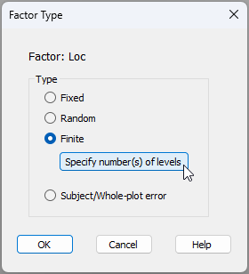
7. Specify any finite factor(s) and provide relevant population-level details - To specify that the 'Location' factor is finite and give further details, first click inside the cell in row 2, column 3 of the design file (shown below).

In the 'Factor Type' dialog window, choose Type > $\bullet$ Finite, and click the button to 'Specify number(s) of levels', like so:

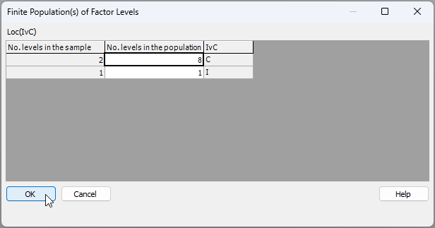
In the resulting dialog window, you will need to articulate the size of the population of levels from which sampled levels have been drawn. PRIMER will already assert (in column 1 below) the number of levels of the finite factor have been sampled, given the name of the factor you have provided. But the number of levels in the population (from which sampled levels have been drawn) cannot be gleaned directly from the data and its associated factor information. So, the researcher has to provide it.

Note also that, in this particular case, the factor of 'Location' is nested in 'IvC'. So we will need to specify the size of the population of levels for each of:

• (i) the control locations (shown in row 1 below); and
• (ii) the impact locations (shown in row 2 below).

We drew $b_1$ = 2 control locations out of $B_1$ = 8, so we should enter '8' for the 'No. levels in the population' for the control state ('C'). There is, however, only one impact location in total ($B_2$ = 1), so we enter '1' for the 'No. levels in the population' for the impact state ('I'), as shown below:

The final completed design file will look like this:

Run the PERMANOVA

When some identifiable fraction of a finite population of possible levels are drawn, the factor can be thought of as somewhere in between fixed and random, and can be analysed explicitly as finite directly within the ANOVA framework. Anderson et al. (2025) have provided (and PERMANOVA+ in PRIMER 8 implements directly) the important methodology to derive expectations of mean squares (EMS) for any ANOVA design having any types of factors along the entire graded progression from fixed to random, inclusive. Furthermore, just as for any PERMANOVA model, tests of hypotheses are carefully achieved here under minimal assumptions of exchangeability, using appropriate permutation algorithms for each term in the model. Inclusion of finite factors merely requires, in each case, the explicit specification of the population size from which observed levels are drawn.

Having specified the full such design for the present case-study, we are now ready to embark on the PERMANOVA analysis itself.

8. Run the analysis - From the 'Resem1' matrix, click PERMANOVA+ > PERMANOVA. Ensuring that the design worksheet is 'Design1', we can take the defaults for the rest and click 'OK'.

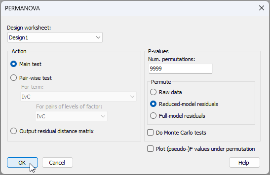
The resulting output file, 'PERMANOVA1', is shown below.

These results show a statistically significant impact of the sewage outfall on assemblages of molluscs along this coastline in the Mediterranean (i.e., for the 'IvC' term, we have $F_{1,5.46}$ = 3.79 and $P$ = 0.021). Also, although there is relatively high site-level variation ($F_{6,72}$ = 4.10, $P$ = 0.0001), there is no evidence for significant location-level variation, over and above this, among the control locations ($F_{1,6}$ = 1.47, $P$ = 0.1972). Note that our inferences here extend to the finite population of 8 locations along the Italian Mediterranean coast from which we have sampled, but not beyond that.

---

^¶There are some rather large abundance values here and, given the relatively large number of replicates per site, these data would be a great candidate for the application of dispersion weighting, as a pre-treatment option. Alternatively, we might think it sensible to apply a fourth-root transformation as a pre-treatment, to downweight the influence of the more abundant species. Here, we have chosen to analyse the data without any transformation or pre-treatment, simply to maintain consistency with the approach taken by Terlizzi et al. (2005) .

---

^†One could also look at (say) a non-metric MDS ordination among all of the original $N$ = 81 replicates. The lowest stress achieved for the 2-dimensional solution is 0.196, which makes it difficult to interpret finer details with much confidence (due to high variation among replicates). Another alternative is to calculate and then plot distances among the site centroids, without doing any bootstrapping; however, on its own, this won't show the variability in those site centroids. We acknowledge that bootstrap routines to examine variation in centroids in the dissimilarity space (rather than averages of the original variables) would be a desirable addition.

---

^‡Note that, for this example, the 'appropriate number of dimensions' in which to do the bootstrapping (by default) turns out to be $m$ = 10 metric MDS axes, which achieves a matrix correlation with the original resemblance matrix of $\rho$ = 0.960. This can be seen in the 'Diagnostics' section of the output file called 'Bootstrap Average1', produced by the Bootstrap Average routine when run with these parameters on this dataset.

---