15.8 Output diagnostic plots from CAP

In PRIMER 8, it is now possible to output diagnostic plots from the CAP routine (i.e., canonical analysis of principal coordinates, an analysis obtained from a resemblance matrix by clicking PERMANOVA+ > CAP). You simply tick the new option to '$\checkmark$Do diagnostic plots' in the CAP dialog window.

For example, consider a study of the assemblages of small benthic fishes living in rocky subtidal reef habitats in northeastern New Zealand, examined by Smith & Anderson (2016) . Data from this study are located in the file called 'NZ_benthic_fish.pri', in the 'Examples_P8' > 'NZ_benthic_fish' folder. Surveys were done of the benthic fish fauna, along with fine-scale habitat features in kelp forests and rocky reefs along the north-eastern coast of New Zealand. There were sites at a range of locations in and around several marine reserves (including Leigh, Tawharanui, Hahei and the Poor Knights Islands), and data were obtained over a period of 3 years (2011-2013). At each site, divers surveyed $n$ = 8 transects, measuring 1 m $\times$ 5 m. Each transect was made up of five contiguous 1 m $\times$ 1 m quadrats. For each quadrat, divers first visually searched and recorded counts for all benthic fishes, then recorded the presence/absence of a set of pre-defined habitat features (see the file named 'NZ_benthic_fish_habitat.pri', located in the same folder).

Here, we shall consider only the potential effects of the marine reserve at Leigh on these fish communities in a fully balanced design. Note that the factor of 'Reserve' has two levels: 0 = outside the reserve, and 1 = inside the reserve. Due to the sparsity of the count data at small spatial scales, we shall analyse data summed to the transect level, then consider densities of each species (averages per transect) at the spatial scale of sites for the ensuing CAP analysis. Mean densities (per 5m²) of each fish species per site are located in the file named 'NZ_benthic_fish_Leigh_av_densities.pri'.

1. Open the file ('NZ_benthic_fish_Leigh_av_densities.pri') in PRIMER 8. It will look like this:

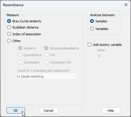
2. From 'NZ_benthic_fish_Leigh_av_densities', click Analyse > Resemblance... and choose to calculate the Bray-Curtis similarity among samples. This will produce a resemblance matrix called 'Resem1'.

3. From the 'Resem1' matrix, run the CAP routine aiming to distinguish small benthic fish communities inside vs outside the marine reserve, by clicking PERMANOVA+ > CAP and choose:
   (Analyse against $\bullet$Groups in factor > Factor for groups or new samples: 'Reserve') &
   ($\checkmark$Scores to worksheet) &
   (Diagnostics > $\checkmark$Do diagnostics > $\checkmark$Do diagnostic plots) &
   ($\checkmark$Do permutation test > Num. permutations: 9999)
   

then click OK, as shown below:

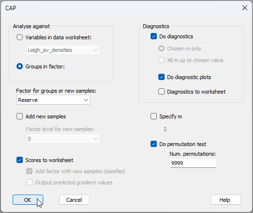
The option to do diagnostic plots is new to PRIMER 8.

The analysis will run and produce the following:

• 'CAP1' (), containing all of the essential results in a rich text format (*.rtf), and
• 'MultiPlot1' (), containing the CAP plot itself (as 'Graph1') along with plots of the diagnostics for choosing $m$, where $m$ = the number of principal coordinate axes (PCOs) used to produce the canonical (CAP) axis (as 'Graph2' through 'Graph5').

From 'CAP1' and the accompanying CAP plot ('Graph1'), shown below, we can see that the canonical correlation associated with the 'Reserve' effect is reasonably strong ($\delta_1$ = 0.644), and that this is statistically significant ($\delta_1^2$ = 0.415, $P$ = 0.001). This CAP model was achieved with $m$ = 4 PCO axes, which achieved a leave-one-out allocation success of 77.78% under cross-validation.

The four diagnostic plots are shown below.

It is clear that the choice of $m$ = 4 is a good one here, as this choice achieved the greatest leave-one-out allocation success ('Graph2') and the lowest leave-one-out residual sum-of-squares ('Graph3'). Although this can also (technically) be seen in the 'DIAGNOSTICS' section of the 'CAP1' output above, it is certainly much clearer to see this information in diagnostic plots, whereby the wisdom of the choice made, overall, by reference to other values of $m$, can be readily assessed.