9.2 Periodic and cyclical models
Natural cycles in biology and ecology
Important situations where the treatment of multiple covariables as a single set would be desirable in PERMANOVA are cases of periodic or cyclical phenomena in biology or ecology. Examples might include:
- seasonal patterns (e.g., monthly or quarterly sampling at temperate latitudes, migrations)
- cyclical reproduction (e.g., spawning aggregations, flowering and fruiting cycles)
- lunar patterns (e.g., tidal cycles, hormonal cycles)
- global climate cycles (e.g., El Niño vs La Niña, North Atlantic Oscillations)
- circadian rhythms (e.g., 24-hr sleep cycles)
All such cyclical phenomena may generate cyclical patterns in multivariate data, and it would be very useful to be able to model these in the space of a resemblance measure, using PERMANOVA. However, as cyclical patterns are not linear, we (generally) need more than one dimension to model them appropriately.
Modeling cyclical phenomena using ANOVA/Regression
A straightforward way to model cyclical phenomena using ANOVA/regression is to use two variables, corresponding to the periodic sine and cosine functions (e.g., Bliss (1958) ). Let's consider modeling a seasonal cycle. There are 12 months of the calendar year, and suppose we have sampled monthly and we label these months from 1 to 12 in our data set. However, we expect that samples taken in month 1 (January) will be more similar to samples taken in month 12 (December) than they will be to those taken, say, in month 6 (June).
Let $k$ be the number of samples we have taken at equal intervals in our cycle.¶ Here, $k$ = 12. For our model, let's imagine that our $k$ = 12 months occupy 12 equally spaced positions along the circumference of a circle with a radius of $r = 1$.† The circumference of a circle can be described as going from 0 all the way around to 2$\pi$ (360 degrees) in radians. With each passing month, we will travel a distance 1/12th of the way around this circle's circumference. So, the distance between each pair of consecutive months, in radians, is $c = 2\pi / k$. Thus, the model position of any given month, $t = 1 ,..., k$, along the circumference of the circle is easily found as $c \times t$.
We might consider using something like a sine (or a cosine) function to model periodic phenomena, as either one of these, on its own, will yield a wave-like pattern over the range from 0 to 360 degrees (that is, from 0 to 2$\pi$ in radians; Fig. 9.1).
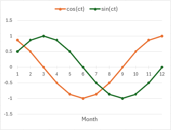
Fig. 9.1 Sine and cosine functions of $ct = 2\pi t / k$ versus twelve equally-spaced positions (i.e., months from $t = 1, ..., 12$) along the circumference of a circle of radius $r = 1$.
However, it is readily seen that using just one of these functions alone will not suffice for our purposes. For example, the value of the sine function is equal to zero at month 6 and also at month 12 (Fig. 9.1), but we obviously do not want the model to consider these as equivalent. Similarly, the value of the cosine function equates (for example) month 3 and month 9, which is also undesirable for us. Thus, any single wave function does not fully capture the full nature of cyclical phenomena.
If we were to take both functions simultaneously, however, we would indeed capture the full circle (Fig. 9.2).
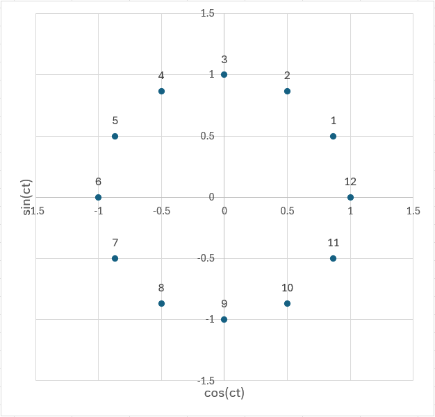
Fig. 9.2 Two-dimensional scatter plot of $\sin(ct)$ versus $\cos(ct)$, showing the 12 months (points) along the unit circle.
In Figure 9.2, we can see that: (i) the 12th month apparently occurs at "3 o'clock" and (ii) the numbers run counter-clockwise, rather than clockwise around the circle. Clearly, neither of these things actually matters in the least for our purposes. We have just created a model of a cycle with 12 equally spaced positions. There is in fact no natural starting or finishing point - the value of 1 follows the value of 12 in the same way that the value of 12 follows the value of 11. Furthermore, and most importantly, the distance between any pair of points in this 2-D space directly reflects, monotonically, the distance in time that would occur between those two months for any 12-month period (cycle) we care to choose.
The most important point here is that we require both of these variables together to create this cyclical picture: namely, $\sin(ct)$ and $\cos(ct)$. This means that if we want to test a model of cyclicity using PERMANOVA, then we will need to include both of these variables as covariables simultaneously. We would treat them together as a single set (with 2 degrees of freedom) and we would want for them to appear as a single line in the PERMANOVA table of results (e.g., with a name like "Seasonal Cycle" or something similar), to permit a test for monthly seasonal cycles. Testing either of these as individual covariables, alone, would clearly not achieve our aim.
We shall demonstrate this analytical approach using the new tool for grouping covariates available in the PERMANOVA routine for PRIMER 8. Our example is a data set with monthly sampling of intertidal macroalgae from Vancouver in British Columbia, Canada.
¶The intervals do not need to be equally spaced. Any intervals can be modeled in this way (i.e., along the circumference of a circle) at whatever spacings are required.
†The radius is irrelevant here; choosing $r$ = 1 is merely convenient.