4.2 Example: Plankton hauls

An example of a paired design with two groups is provided by Snedecor (1946) , who described a study by Winsor & Clarke (1940) to investigate the total catch of five different groups of plankton (hence, five variables, named using Roman numerals I, II, III, IV and V) by 2 nets hauled horizontally behind a boat. One net was 2 metres below the other one. More specifically, ten hauls were made with the pair of nets situated at depths of 29 m and 31 m. The factors associated with these data are:

• Position (either the upper (U) or the lower (L) net); and
• Haul (10 hauls, labeled 1-10).

Clearly, the two nets (upper and lower) being hauled at the same time are ‘paired’ with one another, so the ‘Haul’ factor is the factor identifying the different pairs of samples here. These data are located in the file ‘Woods_Hole_zooplankton.pri’, found inside the 'Examples_P8 > Woods_Hole_zooplankton' folder. Here, we are going to analyse a single variable – the sum of the log abundances of all plankton types. Specifically, we are going to test the null hypothesis that the paired differences between the upper and lower nets are stochastically symmetric about zero (i.e., there is no effect of ‘Position’).

Running the Wilcoxon signed-rank test

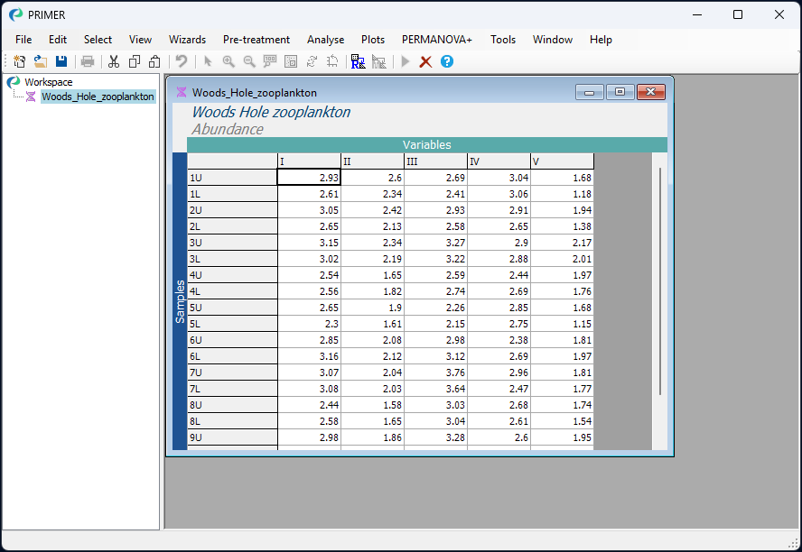
1. Open up the file (‘Woods_Hole_zooplankton.pri’) in PRIMER and note that the abundances are already expressed as log abundance values, so there is no need to apply any transformation.

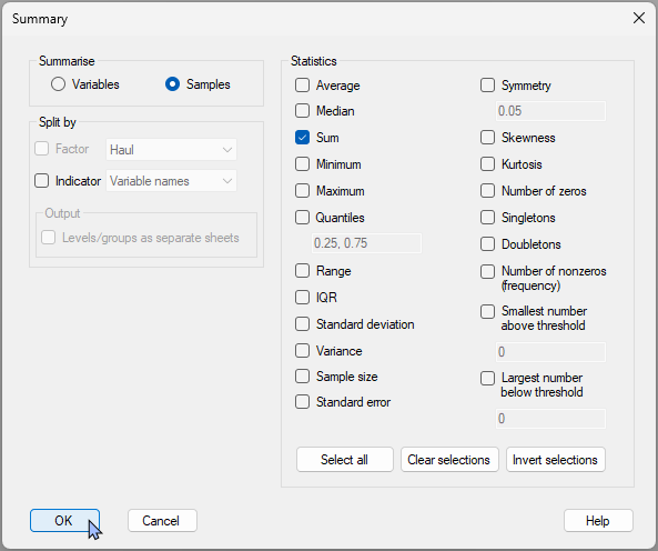
2. Click Tools > Summary Stats… then (Summarise $\bullet$Samples) & (Statistics $\checkmark$Sum), and click ‘OK’. {Note: Be sure to untick the default tickbox, ($\square$ Average), as here we only want to get the sum across the five variables in order to analyse the sum of log abundances across the 5 variables for each sample, as a univariate variable}.

3. The resulting data sheet will be called 'Data1'. From this data sheet, keep things tidy by re-naming the variable from 'Sum' to 'Sum.log.abund'. Click Edit > Labels > Variables… and make this change, as shown below:

4. Let’s now do the test. From ‘Data1’, click Analyse > Univariate > Wilcoxon Signed-Rank…

5. Choose the following in the Wilcoxon Signed Rank Test dialog:
   

then click ‘OK’, as shown below.

Results of the Wilcoxon test

The resulting notepad , *.rtf) file named 'Wilcoxon Signed-Rank Test1' contains all of the essential elements of this analysis and its results. First are shown the choices that were made by the user ('Parameters'):

This is followed by the full suite of results, including all of the relevant supporting calculations ('Results'), viz.:

There was a statistically significant difference between these two nets (upper vs lower) in the sum of log abundances of plankton captured ($W$ = 39, $P$ = 0.0488). Furthermore, the positive value of $W$ indicates that 'Level 1' (which in our case was 'U', the upper net, towed at a shallower depth) typically had larger values than 'Level 2' ('L', the lower net, towed at a slightly deeper depth).

The two graphical outputs from this analysis are:

• 'Graph1 - a histogram of the distribution of values of $W^\pi$ obtained under permutation, showing also the observed value $W_\text{obs}$ (dotted lines):

and

• 'Graph2 - a boxplot of the differences (upper minus lower) in the sum of the log abundance values of these five taxa per haul

The boxplot shows that the median (and indeed the entire inter-quartile range) of the differences in total log abundance is clearly well above zero, consistent with the positive value of $W_\text{obs}$.

Note that this is a two-tailed test. If we wish to postulate a more specific alternative hypothesis, corresponding with the expectation that there will typically be a greater sum of log abundance values of plankton captured in the upper net, we can re-run the analysis precisely as above but with the option:

Alternative hypothesis: Paired differences (level1 - level2) are symmetric around D
          $\bullet$D > 0 (one-tailed test)

That will produce a one-tailed test, which will have greater power. The one-tailed test yields the same value of the Wilcoxon test-statistic as the two-tailed test ($W$ = 39 in this example), but naturally yields a p-value that is half the size of the corresponding two-tailed test (i.e., $P$ = 0.0244 for the one-tailed test in this example).