8.1 Designs lacking replication

In some cases, experiments are done in a way that lacks replication, often at the smallest spatial or temporal scale in the experimental design, but sometimes at larger scales as well. Examples of designs that lack replication include (but are not limited to):

• randomised blocks
• repeated measures
• split-plots (and split-split-plots, etc.)

Randomised blocks

For clarity on what follows regarding 'lack of replication', let's start by considering a simple randomised block design. For example, there might be $a$ = 4 blocks, and within each block, there might be $b$ = 3 treatments randomly allocated to replicates within each block (Fig. 8.1).

Fig. 8.1. Schematic diagram of a randomised block design, with $a$ = 4 blocks and $b$ = 3 treatments randomly allocated to the three replicates within each block.

The number of replicates in each block is equal to the number of different treatments. Thus, there is no replication of the treatments within any of the blocks; i.e., there is only one sampling unit per treatment per block ($n$ = 1). This means that we cannot estimate any component of variation that might be due to a potential 'Treatment x Block' interaction, as it is inextricably confounded with the residual variation (from one sampling unit to the next). In PRIMER, the PERMANOVA routine will recognise this situation automatically. It will issue a warning to highlight this lack of replication, but then it will permit you to proceed with the analysis anyway and simply exclude the 'Treatment x Block' interaction term from the model.

Repeated measures

A similar thing (lack of replication) often happens with study designs that involve repeated measures. Suppose we want to follow the health outcomes for a set of (say) 4 individuals who have taken a drug and another set of 4 individuals that have taken a placebo. We have the factor of 'Treatment' with $a$ = 2 levels (Drug, Placebo), and we monitor the health of our subjects by measuring one or more variables on each individual at a series of time points (time 1, time 2, time 3, ..., time 5). In terms of factors, we therefore also have $b$ = 4 individuals per treatment ('Subject', random and nested in 'Treatment') and $c$ = 5 time-points, but we only have one measurement per person per time point (Fig. 8.2).

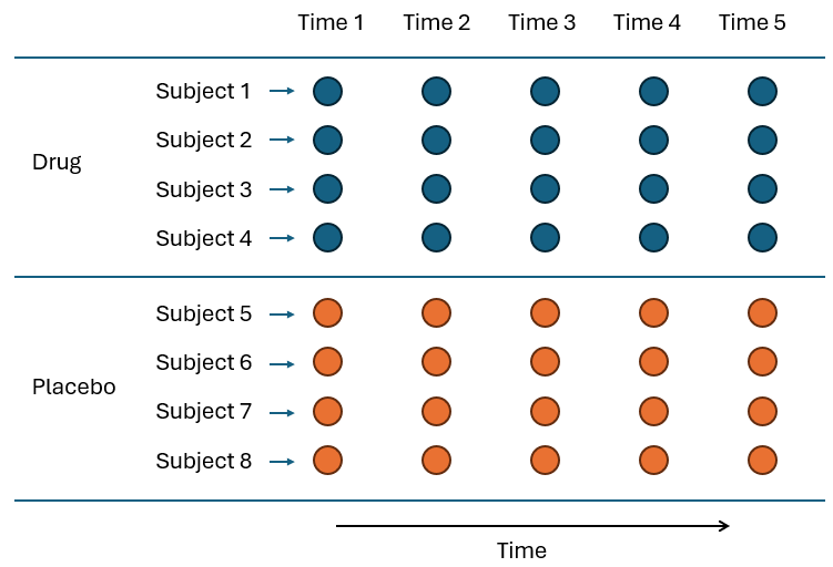
Fig. 8.2. Schematic diagram of a repeated measures design, with $a$ = 2 treatments (Drug and Placebo), administered to each of $b$ = 4 individuals (Subjects) per treatment, who were then each sampled repeatedly through time ($t$ = 1, ..., 5).

We can see there is a similar problem here. The variation due to the potential 'Subject(Treatment) x Time' interaction (if any) is of course inextricably confounded with the residual variation among the sampling units themselves. Once again, just as in the randomised block case, the PERMANOVA routine will recognise this lack of replication and will automatically exclude the 'Subject(Treatment) x Time' term from the model output, after issuing a suitable warning.

Split plots

In some cases, there may be lack of replication not only at the smallest scale, but also at a larger spatial (or temporal) scale in the design. Split-plot designs are classically used in agricultural experiments, where the researcher is interested in investigating more than one factor, but perhaps one of these factors occurs at (or must be manipulated or administered at) a larger scale than others. A typical example might be a study of the effects of irrigation and nutrients on the growth of corn (maize). Different irrigation levels might need to be applied to large areas (fields) due to the equipment and logistics involved, while fertilizers providing different nutrient levels can be applied to smaller areas (plots) within the fields having differing levels of irrigation.

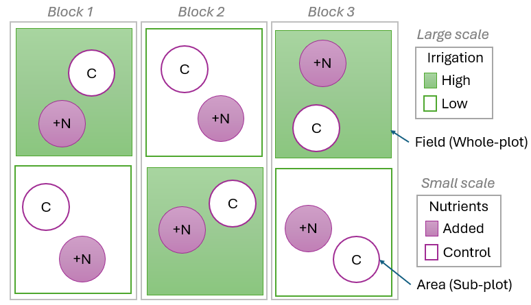
Fig. 8.3. Schematic diagram of a split-plot design, where irrigation levels are administered at a large scale (i.e., to whole-plots), and nutrient levels are administered at a small scale (i.e., to sub-plots).

In such cases, we may think of the design as having two different 'error' terms to consider: one at the level of 'whole-plots' (the fields in this example) and one at the level of sub-plots. If we look just at the 'irrigation' factor in this example, it appears precisely like a randomised block design at a large scale: there are 3 blocks and the two irrigation treatments are applied to two large-scale whole-plots in each block. Thus, when we test the effects of irrigation, the variability from one whole-plot to another is the appropriate 'error' term to consider. In turn, when we investigate the effects of nutrients, we clearly need to consider the variability from one sub-plot to another as our 'error' for that test.

A proposed rationale for using a split-plot design is that factors may occur naturally at different scales (e.g., Mead (1988) ). Another proposed rationale is that one may already know that factor A (at a large scale) has important effects, and one may be willing to sacrifice information on factor A to get more precise results for factor B and the interaction A $\times$ B. For more information regarding the assumptions and potential disadvantages of split-plot designs, see Mead (1988) and Underwood (1997) .

New factor type: Subject/Whole-plot

The new PERMANOVA routine in PRIMER 8 caters well to repeated measures and split-plot designs directly. Specifically, there is a new 'Factor Type' called 'Subject/Whole-plot error', as shown below:

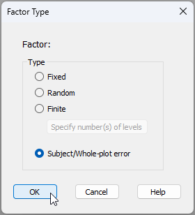
This is ideal for situations where entities (plots, individuals, subjects) are sampled multiple times (as in repeated measures), or cases where different treatments are administered at different spatial scales (e.g., to whole-plots and sub-plots in split-plot designs) in a way that lacks replication (at whatever scale). These types of study designs represent special cases where there may be insufficient replication to estimate all of the potential interactions among factors genuinely implied by the full set of factors in the study.

Previous versions of PERMANOVA for PRIMER would handle cases lacking replication within the highest-order cells by issuing a warning and excluding/removing the highest-order interaction (as indicated above for the randomised block and repeated measures cases). This strategy, however, does not handle situations where the confounding occurs somewhere else in the study design (e.g., at larger spatial scales), as it typically does for a classical split-plot design. In such cases, historically, when using PERMANOVA (in version 6 or version 7 of PRIMER), the end-user had to figure out which terms (if any) should be excluded from the model, and then would have had to exclude them manually (using the 'Terms' button). Failure to do this could result in certain terms in the model appearing with the words 'No test' in the output.

Basically, PERMANOVA in PRIMER 7 does not directly cater to the situation where you have (effectively) a nested term that also lacks replication and that occurs at a different level in the design (e.g., at the level of 'whole plots'). The specification of a whole-plot (or subject) type of factor can be thought of like the specification of an additional error term that occurs at a larger spatial scale than the scale of individual replicates.

Thankfully, the new PERMANOVA routine in PRIMER 8 handles these types of factors and designs easily, directly and correctly.