6.6 Example: one-way PERMANOVA allowing heterogeneity

Let's look now at an example where there is a single factor in the study design, the number of replicates per group is unequal and there is clear heterogeneity in multivariate dispersions among the groups. Ellingsen & Gray (2002) studied the biodiversity of soft-sediment macrobenthic organisms and its relationship with environmental variation over large spatial scales in the North Sea. Samples of soft-sediment macrobenthic organisms were obtained from $N$ = 101 sites occurring in five large delineated areas along a transect spanning 15 degrees of latitude (Fig. 6.4). The sample sizes in the five areas were: $n_1$ = 16, $n_2$ = 21, $n_3$ = 25, $n_4$ = 19 and $n_5$ = 20. A total of $p$ = 809 taxa were recorded overall, and samples consisted of abundances pooled across five benthic grabs obtained at each site.

Interest lies in comparing the multivariate assemblages of organisms occurring in these five areas. More specifically, we wish to use PERMANOVA to test the null hypothesis:

• H₀: there are no differences in the centroids of these 5 areas in the space of the Jaccard resemblance measure, allowing for any potential heterogeneity in the within-group dispersions among these areas.

In ecology, the Jaccard measure is directly interpretable as the percentage of shared species between every pair of sampling units. When expressed as a dissimilarity, it is often used as a pure measure of turnover in studies of beta diversity ( Anderson et al. (2006) ).

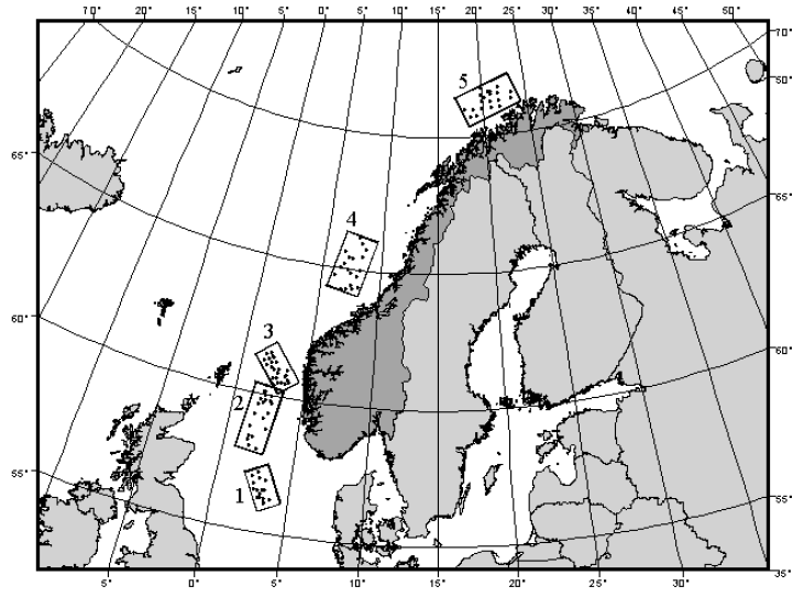
Fig. 6.4. Map showing locations of sites in each of 5 areas in the North Sea from which macrobenthic fauna were sampled (after Ellingsen & Gray (2002) ).

Open the data in PRIMER and examine patterns

1. Start running PRIMER 8, then click File > Open... to open the data file named 'Norway_macrofauna.pri' (found inside the 'Examples_P8 > Norway_macrofauna' folder).

2. Get the resemblance matrix among the sampling units based on the Jaccard measure. Click Analyse > Resemblance... > (Measure > $\bullet$ Other) and from the drop-down list choose 'S7 Jaccard'.

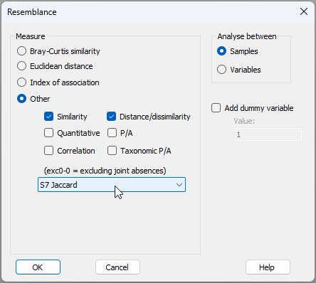
The resulting resemblance matrix will be called 'Resem1'.

3. To visualise the inter-sample relationships based on the identities of the fauna they contain, obtain a non-metric multi-dimensional scaling (nMDS) ordination plot based on the Jaccard resemblances. From the 'Resem1' similarity matrix, click Analyse > MDS > Non-metric MDS (nMDS)..., take the default options and click 'OK'. This will generate the following 2D ordination plot (called 'Graph1'), or a highly similar solution^¶:

Perhaps the most striking pattern here is the tight clustering of samples from Area 1 (low dispersion) and the very large spread of the samples from Area 3 (high dispersion), compared to Areas 2, 4 and 5.

Test for homogeneity of multivariate dispersions

4. Although it is fairly obvious from the graphic, let's test the null hypothesis of no differences in the within-group dispersions among the five areas using PERMDISP. From the 'Resem1' similarity matrix, click PERMANOVA+ > PERMDISP... > Group factor: Area (leaving the rest as their defaults) and click 'OK', as shown below:

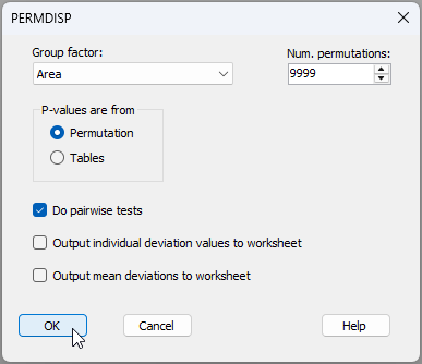
The results are given in the file 'PERMDISP1' of the Explorer tree (see below).

There are clearly highly significant differences in the dispersions among the groups ($F$ = 49.778, $P$ = 0.0001 with 9999 permutations). The pairwise tests, furthermore, reveal how Area 1 and Area 3 differ significantly from one another and from the other three groups (2, 4 and 5) with respect to their dispersions, reflecting rather directly the patterns of differences in spread we observed in the nMDS plot.

Test for differences in centroids, allowing for heterogeneity

Having observed these dispersion differences among the areas - quite interesting differences in themselves - we now aim to test for diferences in centroids, allowing for that heterogeneity. Running a PERMANOVA requries two steps: (i) setting up a design file; and (ii) running the PERMANOVA analysis on a given data set in response to a specified design.

5. From the 'Resem1' similarity matrix, create the design file by clicking PERMANOVA+ > Create PERMANOVA Design.... You will see a new item named 'Design1' (symbolised by ) in the Explorer tree. You will need to do the following:

• Click the white cell in the first column under the word 'Factor' and choose: 'Area' as the sole factor of interest for this design. (Note in passing that the default is to treat this factor as 'Fixed', as shown under the word 'Type' in the third column of the design file, which is fine here).
• Under 'Dispersions', tick the box $\checkmark$ 'Allow for heterogeneity', then click the button.
• In the resulting dialog box entitled 'Select the term identifying groups with different dispersions' choose 'Area'.

Your resulting design file should look like this:

Note that by ticking the box $\checkmark$ 'Allow for heterogeneity', we ensure that the PERMANOVA tests will be done using $F_2$ rather than $F_1$ for all tests of relevant terms affected by the heterogeneity we have identified using the 'Groups' button.

6. Now that you have created the design file, you are ready to run the analysis itself. We're going to test the null hypothesis of no differences in the centroids among the five areas using PERMANOVA and allowing for heterogeneity in dispersions. Go back to the 'Resem1' similarity matrix and, from there, click PERMANOVA+ > PERMANOVA.... In the PERMANOVA dialog window:

• Under the words 'Design worksheet:' make sure you choose the name of the correct design file, i.e. 'Design1'.
• Under the word 'Action', choose $\bullet$ Main test.
• Under the word 'Permute' choose $\bullet$ Raw data (because there is only one factor here).
• Optionally, you can choose to tick the box to $\checkmark$ 'Plot (pseudo-)F values under permutation'. The rest of the items in the dialog can remain as the defaults (see below), then click 'OK'.

The resulting PERMANOVA output file ('PERMANOVA1', shown below) indicates strong evidence against the null hypothesis of no differences in the centroids among these five areas ($F_2$ = 13.51, $P$ = 0.0001 with 9999 permutations). So, not only are there differences in the variability of the assemblages (evidenced by the PERMDISP analysis), there are also clear shifts in centroid evidencing overall turnover in the identities of species across these five areas (also apparent in the nMDS plot above).

It is worth noticing a couple of things about the PERMANOVA output file that makes it different from what would be obtained if we did not allow for heterogeneity. Specifically:

• The expectation of the mean square for 'Area' includes linear combinations involving separate individual measures of residual variation for each of the five areas. In other words, we do not have a single pooled estimate of error variance at work here, but an explicit recognition of the different within-group dispersions.
• The denominator degrees of freedom for the test of 'Area', therefore, is not a whole number, but instead this value is drawn directly from the theory for this arising from the univariate solution to the Behrens-Fisher problem described by Brown & Forsythe (1974) . As previously discussed, this has no direct consequence on the test by permutation using $F_2$ for the multivariate setting, but it does point to the fact that the power of the test using $F_2$ may well differ from that using $F_1$ (which perfectly stands to reason, as they are actually testing different hypotheses).

7. Having found a significant result for the main test in PERMANOVA, it is now desirable to run pair-wise comparisons that also will account for heterogeneity. We simply re-run the PERMANOVA routine from the same resemblance matrix, pointing to the same design file ('Design1'), but this time, under the word 'Action', we choose $\bullet$ Pair-wise test > For term: 'Area' > For pairs of levels of factor: 'Area', like this:

Our results file for the pair-wise tests ('PERMANOVA2') will then appear as follows:

In passing, we can see how using $F_2$ on the pairwise tests creates differences from what we would see for a PERMANOVA using $F_1$ on these data. These differences essentially mirror what we saw for the main test; namely, there are separate individual measures of residual variation for each area, and there are also non-integer denominator degrees of freedom for each test.

Overall, from this study, we can conclude that there are highly significant differences in the identities of species obtained from each of these five different areas - they clearly contain different sorts of soft-sediment benthic assemblages. This is so despite the very large variation in the assemblages inhabiting different sites sampled from Area 3. Our tests accounted for that.

It is obviously very satisfying to be empowered by the new PERMANOVA routine in PRIMER 8. We can now make statistically rigorous inferences about differences in centroids in the space of a chosen resemblance measure that allows for heterogeneity.

---

^¶If your plot looks different, it is probably because of an arbitrary rotation or perhaps a 'flipping' of the X axis and/or the Y axis. Any nMDS results shown in an ordination diagram are invariant to changes in the signs of the axes and hold equivalent information for interpretation (preserving as they do the rank-order inter-relationships among the points). You can 'flip' either axis by right-clicking anywhere on the plot (to bring up the 'Graph' menu) and then click 'Flip X' and/or 'Flip Y'.