13.4 Example: Gulf of Maine invertebrates - functional resemblance

There are many situations where the standardisation of samples is required as a pre-treatment prior to analysis, but which needs to be done separately within groups of variables that may be identified by an indicator.^¶ Here, we shall consider a dataset comprised of occurrences of $p$ = 91 macroinvertebrate species recorded from intertidal areas at each of $N$ = 12 exposed rocky headlands (surveyed in 2012) in the Gulf of Maine (Fig. 13.3, Trott (2022) ^†). For each species, we have additional information in the form of trait data. The trait data for each species consists of presence/absence information for a series of $q$ = 93 individual trait variables. The trait variables are organised into 14 groups. These groups of traits are: Form, Position, Lifestyle, Trophic Relation, Body Shape, Body Support, Flexibility, Ecoengineer, Fertilization, Development, Size, Body Plan, Asexual Reproduction and Regeneration. The number of categories (trait variables) within each trait group varies, and any given species can be recorded as a '1' (indicating that they belong) to one or more of these categories within each trait group.

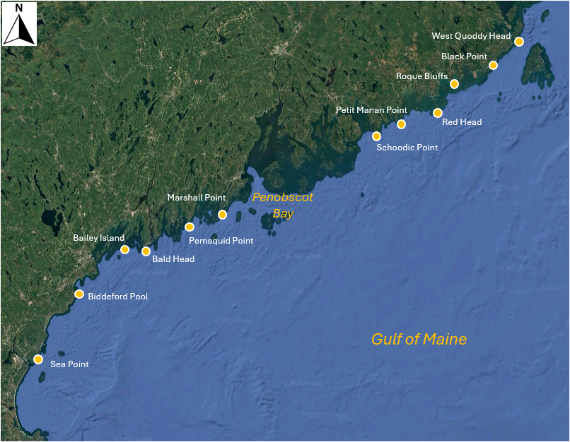
Fig. 13.3 Map of the Gulf of Maine showing 12 sites where macroinvertebrates were sampled by Trott (2022) . Satellite image: Google Earth.

Our initial agenda here may be to consider the relationships among the sites based on the species they contain in the usual way, e.g., using the Bray-Curtis (or Sørensen) resemblance measure directly on the species $\times$ site matrix. However, we may wish to nuance this calculation further by incorporating relationships among the species, based on their traits. In other words, if two sites do not share any species in common, they might nevertheless share two species that have similar traits. We can exploit the method of calculating taxonomic resemblance ('Gamma+', Clarke et al. (2006b) ) in order to calculate, instead, a functional resemblance, using a matrix of inter-species relationships built from the trait data (e.g., Myers et al. (2021) ).

Further to this aim, we shall consider our trait data matrix such that the classical role of 'samples' is given to the species (among which we shall calculate the resemblances), while traits are given the role of 'variables'. However, we want each trait group to be weighted equally in the calculation. To make sure the sum of values for each species within each trait group sums to 100 (so gets equal weight), we will want to apply a pre-treatment to standardise across the trait variables for each species ('sample'), but separately within each trait grouping. This standardisation would not be necessary if every species only had one trait within a group, but that is not the case here. For example, the mollusc species, Adalaria proxima (abbreviated ADP) is in two trophic categories: it grazes on algal fronds and blades (Tr-P-GF), and also grazes macro prey on the substratum (Tr-P-GSM).

Our analysis pathway looks like this:

• Open the trait data matrix in PRIMER 8.
• Standardise the 'samples' (species here) across the trait variables, separately within each trait grouping, using our new tool in P8, Pre-treatment > Standardise....
• Calculate functional resemblances among species using Bray-Curtis, based on the standardised trait data.
• Examine the inter-species functional relationships in an ordination (nMDS).
• Calculate functional resemblances among the 12 sites, by incorporating these species inter-relationships.
• Examine the functional relationships among the sites in an ordination (nMDS).

Open the trait data matrix

1. In PRIMER 8, click File > Open... and open up the file named 'Gulf_of_Maine_invert_traits.pri' (found in the 'Gulf_of_Maine_inverts' folder inside the 'Examples_P8' folder), as shown below.

Note here that the 'Samples' are actually the species (the names are abbreviated). More information about the species can be seen by clicking Edit > Factors.... Note also that the traits are variables. More information about the traits (also abbreviated) can be seen by clicking Edit > Indicators....

The first trait group is actually the name of the Phylum for each species. These are not actually traits, so let's start by selecting all of the traits that do not belong to the 'Phylum' group.

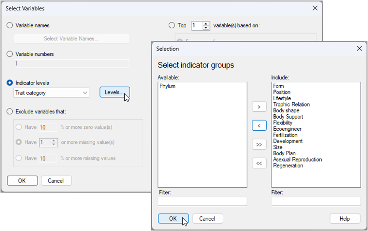
2. From the 'Gulf_of_Maine_invert_traits' matrix, click Select > Variables..., then choose ($\bullet$Indicator levels Trait category) and click the 'Levels...' button (). In the Selection dialog, first click the double right arrows button () to move all of the groups to the 'Include' column on the right. Then click on 'Phylum' and the left arrow button (), so that it appears back in the 'Available' column on the left (as shown below), then click 'OK' (in both dialog windows).

This will create a dataset that is re-coloured with a blue background, showing only the selected subset of traits (excluding 'Phylum'), like this:

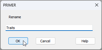
Any analyses from this matrix will now only be done on the sub-setted data. To keep things tidy, click Tools > Duplicate and the subsetted data will now be provided in the Explorer tree as a new matrix called 'Data1'. We can re-name this to 'Traits' by clicking File > Rename Data and typing in this desired new name, then clicking 'OK', as shown below.

Standardise the trait data

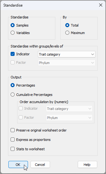
3. From the 'Traits' data sheet, click Pre-treatment > Standardise... and choose (Standardise $\bullet$Samples) & (By $\bullet$Total) & (Standardise within groups/levels of $\checkmark$Indicator Trait category) & (Output $\bullet$Percentages), then click 'OK', as shown below.

The resulting data sheet (called 'Data1') can be renamed (using File > Rename Data, as we have done before) to (say) 'Standardised Data', for clarity. The standardised trait data sheet will look like this:

Note how the distribution of traits within a species for any particular trait group (in this example, the trait groups are identifiable by reference to the letters appearing before the dash '-' in the variable names, e.g., 'Po', 'Li', 'Tr', etc.) will sum to 100.

Calculate relationships among species based on traits

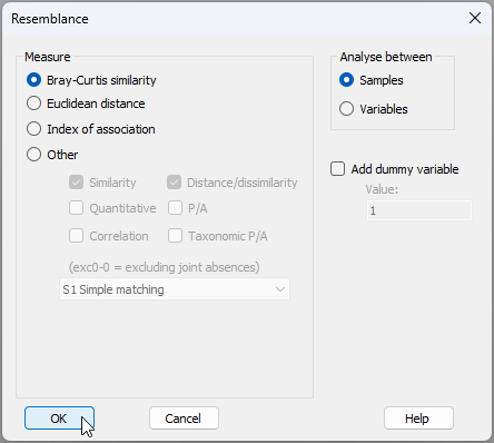
4. From the 'Standardised Data' sheet, click Analyse > Resemblance... > (Measure $\bullet$Bray-Curtis similarity) & (Analyse between $\bullet$Samples), as shown below.

The resulting resemblances among the species, based on their traits is shown below.

We mustn't forget that the role of 'samples' is being taken by the species here! (The traits were the variables that created this matrix). However, in subsequent analyses to follow, the species will be variables, and sites will be samples. So let's go ahead and change the properties of this resemblance matrix now.

From 'Resem1', click Edit > Properties... and change the following:

• Title 'Gulf of Maine invertebrates'; and
• Between $\bullet$Variables then click 'OK' (as shown below).

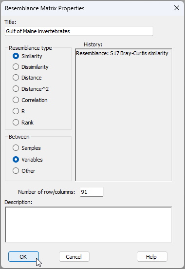
We now have a resemblance matrix among the species which are clearly identified as variables, hence that is ready for ensuing analyses (see below).

As a next step, let's aim to visualise similarities among species, based on their traits, using a non-metric MDS ordination.

Visualise inter-species trait-based relationships

5. From 'Resem1', click Analyse > MDS > Non-metric MDS (nMDS)..., and go with all of the default options in the dialog (just click 'OK'). The resulting 2D ordination ('Graph1' in the Explorer tree) is shown below. Different symbols/colours show the different phyla in which individual species (labeled by their abbreviations) belong.

This ordination has rather high stress (0.214), so we might opt to examine the 3D graphic ('Graph1' in the Explorer tree), which has a lower stress (0.138), as shown below. In essence, this ordination shows us the relationships among these invertebrate species in multi-dimensional trait space.

Next, we shall use these trait-based relationships among the species to inform the analysis of functional turnover among the sites, based on the species they contain.

Calculate functional resemblances (Gamma+) among sites

6. First, we need to open up the species $\times$ site matrix of presence/absence (occurrence) data in the same workspace (click File > Open...). This file is called 'Gulf_of_Maine_invert_occurrences.pri' (also found in the 'Gulf_of_Maine_inverts' folder inside the 'Examples_P8' folder).

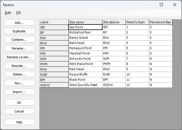
The sites have abbreviated names. Full names (as shown in the map in Fig. 13.3 above) can be seen by clicking on Edit > Factors.... You will also see that the sites have been given a rank ordered value for their position along the Maine coastline ('West to East'), and have also been classified as occurring either north or south of Penobscot Bay, viz:

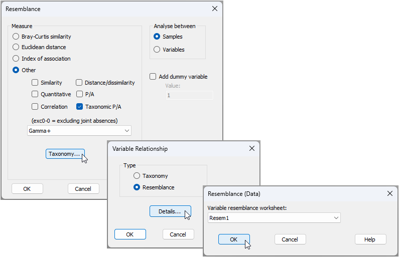
7. Now we shall calculate functional (trait-based) resemblances (Gamma+) among the sites. From the 'Gulf_of_Maine_invert_occurrences' worksheet, click Analyse > Resemblance..., and in the 'Resemblance' dialog window:
   • Choose (Analyse between $\bullet$Samples) & (Measure $\bullet$Other > $\checkmark$ Taxonomic P/A > Gamma+), and click the 'Taxonomy...' button ().
   • In the 'Variable Relationship' dialog window, choose (Type $\bullet$Resemblance), and click the 'Details...' button ().
   • In the 'Resemblance (Data)' dialog, choose (Variable resemblance worksheet: Resem1).
   • Click 'OK' (3 times, once for each successive dialog window) to complete the operation. The dialog windows involved in this operation (i.e., to calculate Gamma+ on the basis of a resemblance matrix, which in our case is a trait-based resemblance matrix) are shown below:

The resulting resemblance matrix of Gamma+ values among the sites (called 'Resem2') is shown below.

Visualise functional turnover among sites

8. We can now easily do an ordination (or indeed a cluster analysis or any other resemblance-based analysis) of the trait-based turnover among the sites. From 'Resem2', click Analyse > MDS > Non-metric MDS (nMDS), just keep all of the defaults and click 'OK'.

9. From the resulting 2D nMDS ordination graphic (called 'Graph5' in the Explorer tree), click Graph > Sample Labels & Symbols... and choose to display labels by the factor of 'Site name', and symbols by the factor of 'Penobscot Bay', as shown in the dialog below, then click 'OK'.

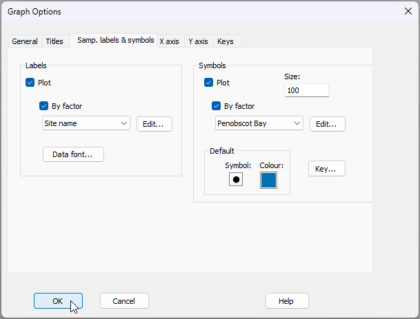
The resulting nMDS graphic looks like this:

This plot shows there is a clear shift in functional traits of intertidal assemblages from sites located to the south (blue symbols) vs those located to the north (amber symbols) of Penobscot Bay. We can do statistical tests of relevant hypotheses about this using ANOSIM (from 'Resem2', click Analyse > ANOSIM...). Doing this shows that:

• This shift is statistically significant (one-way unordered ANOSIM of the factor 'Penobscot Bay', $R$ = 0.546, $P$ = 0.0022); and
• There is a significant sequential change in trait-based relationships among these communities along the coastline (one-way ordered ANOSIM of the factor 'West to East', $R^O$ = 0.422, $P$ = 0.0026).

---

^¶Equally, and in a directly analogous fashion, there are situations where the standardisation of variables is required as a pre-treatment prior to analysis, but which needs to be done separately within groups of samples that may be identified by a factor.

---

^†See also the following abstract by Thomas J. Trott, highlighted in the 4th World Conference on Marine Biodiversity: 'Traits matter: when rarity means more than abundance to functional diversity'.