14.2 Example: NE Pacific groundfish vs depth

To demonstrate the creation and use of ordered groups from a continuous variable, we will look at data comprised of an excerpt from the West Coast Groundfish Bottom Trawl (Slope and Shelf Combination) Survey, conducted annually by the National Oceanic and Atmospheric Association (NOAA)'s Northwest Fisheries Science Center^¶ and available online (https://www.nwfsc.noaa.gov/data/map). This specific excerpt was created and used by Anderson et al. (2022) and is also available on Dryad. Data are provided from trawl surveys for the years from 1999-2018 inclusive. There are two data sheets referred to here (both are found in the Examples_P8 > NE_Pacific_groundfish folder), namely: (1) counts of abundances of $p$ = 310 species of groundfish obtained in each trawl (in the file called 'NE_Pacific_groundfish.pri') and (2) values for latitude, longitude, depth (in m) and the area swept per trawl (in the file called 'NE_Pacific_env.pri').

In this example, there are $N$ = 6002 (!) rows of data (sample trawls), with depth values from 24 m - 1,428 m, and latitudes from 32°N to 48°N. Constructing a nMDS ordination plot of these fish assemblages for all 6002 samples is unlikely to be helpful here! To make some sense of these data that span such large latitudinal and depth ranges, it would be helpful to create some groups of samples occuring at similar depths (and also groups of samples occurring at similar latitudes, e.g., see Anderson et al. (2013) ). Here, we shall focus purely on creating ordered groups of samples from the variable of depth. More specifically, our interest lies in uncovering potential changes in the structure of fish assemblages along the depth gradient.

Open file and create ordered depth groupings

1. Open up the file called 'NE_Pacific_env.pri' in PRIMER 8. It will look like this:

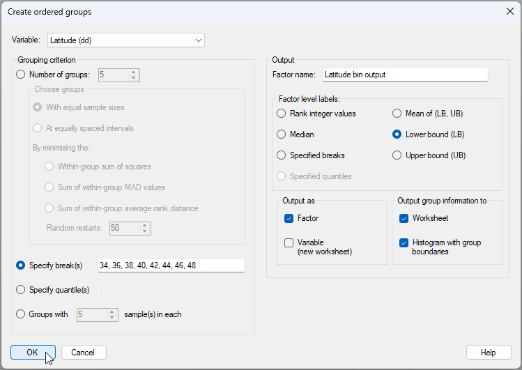
2. From the NE_Pacific_env data sheet, click Tools > Create Ordered Groups..., like so:

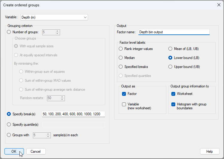
3. In the resulting dialog, choose:

• Variable: Depth (m)
• Grouping criterion > $\bullet$Specify break(s) 50, 100, 200, 400, 600, 800, 1000, 1200
• Output >
  • Factor name: Depth bin output
  • Factor level labels: $\bullet$Lower bound (LB)
  • Output as $\checkmark$Factor
  • Output group information to ($\checkmark$Worksheet) & ($\checkmark$Histogram with group boundaries)

The dialog with these choices will look like this:

Output from the 'Create Ordered Groups...' tool

The output file () called 'Ordered Groups1' in the Explorer tree, has some useful information about how the groups were created. For each group we can see: the minimum, median, maximum, lower bound (LB) upper bound (UB), the mean of (LB) and (UB), and the number of samples that fell into each group. This output file is shown below:

(As an aside, note that we opted in this example also to output this information to a separate data sheet as well, which is called 'Data1' in the Explorer tree.)

Another important part of our output (called 'Graph1' in the Explorer tree) is a histogram of the 'Depth (m)' variable, with the values for the breaks separating the groups shown as vertical dotted lines (as shown below). This is a really helpful way to see the groupings we obtained by reference to the full distribution of sample values for the variable of interest.

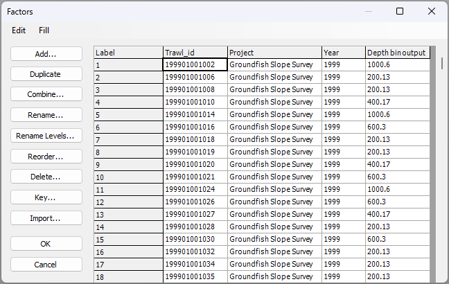
Another thing we get (and perhaps the most useful 'handle' for subsequent analyses we may want to do) is a new factor that is now associated with our original data file. To see this factor, click on the NE_Pacific_env data sheet in the Explorer tree, then click Edit > Factors.... In the 'Factors' window, you will now see this new factor, called 'Depth bin output', provided as the last column (on the right), like this:

Tweak the factor level names (optional)

We asked for the lower bound value of each group to be made the factor level names of our groups, but we can see that these are not necessarily whole numbers. It might be nice to round these to the appropriate whole number, in each case.

4. First, let's duplicate the newly created factor. From the NE_Pacific_env data sheet, click Edit > Factors.... In the 'Factors' window, click anywhere in the column named 'Depth bin output', then click the 'Duplicate' button ().

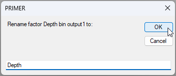
5. You will get a new column with a duplicate factor called 'Depth bin output1'. Click anywhere in this new column, then click the 'Rename...' button (). Rename this factor simply as 'Depth', then click 'OK'.

6. Now we are going to rename the levels of this factor called 'Depth' to whole numbers. Click the 'Rename Levels...' button ().

In the 'Rename Factor Levels' dialog (new to PRIMER8!), you will see two columns: the 'Existing Level Name' on the left and the 'New Level Name' on the right. Change the values in the 'New Level Name' to the desired values , and click'OK', as shown below.

In our case, we have specified new factor level names that are still numeric and consist of whole numbers that will make sense for us in this example for plots/symbols, etc. But note that this tool can be used to re-define the factor level names to anything we wish (not necessarily numbers). Note also, for this example, that we have to be careful not to do too much 'rounding'. We need to stay true to what we know about the data and the bounds of the groups we have created. Bear in mind that we could have changed the names of these factor levels to ranges of depths (e.g., such as 50-100m), which may be better (or more accurate). However, if we change these names to ranges in this way, then we no longer have a strictly numeric factor. Factor levels that are numeric can be really useful in PRIMER, because they allow us to do things like treat the factor as ordered in an ANOSIM, or superimpose trajectories to connect consecutive depths on an ordination plot, etc. In this example, given the new names we have chosen, whenever we describe this factor we will have to be clear what the labels mean; specifically, that the group that we have named '50' here corresponds to samples that occurred between 50 m and 100 m in depth, and so on.

Create a factor for Latitude

We can repeat the above steps for another important spatial factor here: namely, latitude.

7. From the 'NE_Pacific_env' data sheet in the Explorer tree, click Tools > Create Ordered Groups..., then choose to create ordered groups from the variable of 'Latitude (dd)', and specify the breaks to occur in 2-degree increments: {34, 36, 38, 40, 42, 44, 46, 48}, as shown below.

A histogram showing the break-points for latitude that we have chosen is shown below ('Graph2' in the Explorer tree).

8. You will want to tweak this new factor for Latitude (just as we did for the Depth factor before). From the NE_Pacific_env data sheet, click Edit > Factors..., then proceed to do the following:
   • Duplicate the factor of 'Latitude bin ouput' to get 'Latitude bin ouput1' ().
   • Rename the factor 'Latitude bin ouput1' to call it 'Latitude' ().
   • Rename the levels of the factor 'Latitude' to whole numbers (). An image of this last operation is shown below.

Open the groundfish data and import the new factors

Now that we have the factors we want, it would be great to use this to our advantage in analyses of the groundfish data. First we will get the fish data into the workspace, then we will import the new factors (currently associated wtih the environmental data sheet) over to the groundfish data sheet.

9. In the same PRIMER workspace, click File > Open... and open the file called 'NE_Pacific_groundfish.pri'. It will look like this:

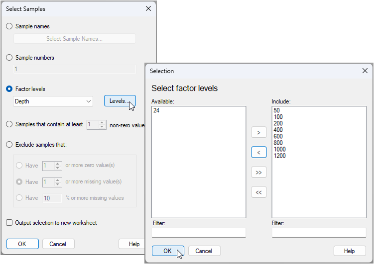
10. From the 'NE_Pacific_groundfish' data sheet in the Explorer tree, click Edit > Factors... and click the 'Import' button (). Choose to import from the 'NE_Pacific_env' worksheet, then click the 'Select' button (). In the selection dialog, pick only the two factors named 'Depth' and 'Latitude' to include in the import, then click 'OK', like so:

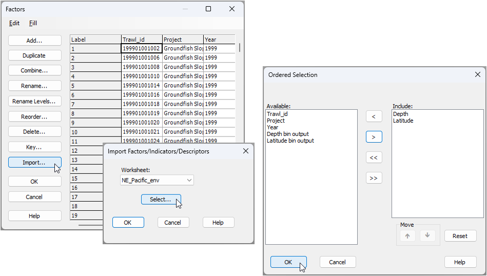
You can confirm that the groundfish sheet now has the 'Depth' and 'Latitude' factors, imported from the environmental data sheet.

Create a combined factor of depth-by-latitude

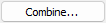
11. For our analysis and plots, we will want now to create a factor that corresponds to the combination of all depth-by-latitude bins. From the 'NE_Pacific_groundfish', click Edit > Factors..., then click the 'Combine' button (). In the 'Combine Factors' dialog, click on the 'Factors...' button (), then in the 'Ordered Selection' dialog, choose to include just Latitude and Depth, as shown below, then click 'OK' (3 separate times for the three windows).

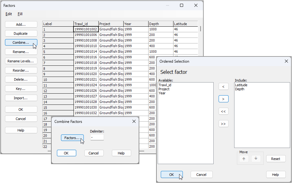
We now have a factor that identifies groups of samples with similar latitude and depth. This new combined factor of 'Latitude-Depth' effectively corresponds to spatial 'cells' of practical interest in our study design, and it will serve us very well for subsequent analyses. (It is the final column on the right in the image below):

Analyse changes in groundfish assemblages vs depth and latitude

We now wish to analyse potential changes in groundfish assemblages with shifts in depth and latitude. Our plan will be to apply a suitable pre-treatment to the data, calculate averages wtihin each latitude-by-depth cell, proceed with calculating a square-root transformation of the data and Bray-Curtis resemblances among these cells, followed by an ordination (nMDS) and tests of hypotheses (ANOSIM) on that resemblance matrix. Note that the averaging step is really important here. We would have no hope of seeing any sensible patterns if we were to 'throw' the full dataset of over 6000 replicates into a single nMDS plot!

Pre-treatment

To analyse the groundfish data, it is appropriate to consider that many fish species occur in clusters or aggregations of individuals. Hence, a pre-treatment option such as dispersion weighting ({{2954#bkmrk-clarkeetal2006a}}) would likely be a really appropriate option here. We shall consider the replicate trawls within each latitude-by-depth cell as fairly natural groupings to use in order to apply this pre-treatment option. We noted that there were only 8 replicate trawls from depths less than 50 m, so we will omit those replicates in what follows.

12. From the 'NE_Pacific_groundfish' data sheet, click Select > Samples... > ($\bullet$Factor levels > Depth), click the 'Levels' button (), then choose to retain all depth groups except '24', and click 'OK', as shown below:

This will turn the worksheet cells blue, and this indicates that a subset of the data has been selected.

13. From this subset-selected groundfish data sheet, click Pre-treatment > Dispersion Weighting... and choose to do this on the basis of the factor 'Latitude-Depth', then click 'OK', like so:

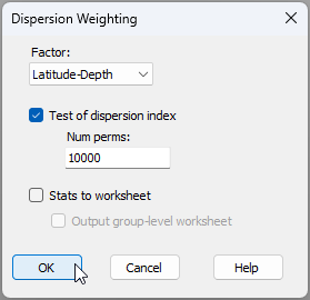
This operation will take some considerable time, simply because of the sheer size of the dataset. The randomization test (for which the individuals of each species are randomly re-assigned to replicates wtihin each of the latitude-depth cells), which is done indpendently for every species, is computationally demanding. However, the results file from the dispersion-weighting pre-treatment (called 'Dispersion weighting1') demonstrates very clearly that many of these fish species show significant clustering (i.e., wherever the value in the 'Divisor' column is greater than 1), hence should sensibly be pre-treated in this way. The dispersion-weighted data is called 'Data3' in the Explorer tree and will look like this:

Averaging

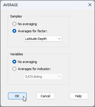
14. From the dispersion-weighted data ('Data3'), click Tools > Average... and choose to average the samples by the factor of 'Latitude-Depth', like so:

In the resulting data sheet (called 'Data4'), we now have average values for each species in each latitude-by-depth cell (rows), as shown below:

Note that the names of the samples in the averaged data now correspond to the latitude-by-depth bin combinations. If you click Edit > Properties..., you will see that this sheet now has 71 rows. We have consolidated these data in a very useful way across our study design, while maintaining the integrity of the underlying information.

Transformation & resemblance

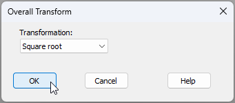
If we look at a shade plot of the averaged data (you can do this by clicking on Plots > Shade Plot... from 'Data4'), we can see that, even after dispersion-weighting and averaging, these data still look pretty sparse. We will therefore do a (mild) overall transformation to square roots, then calculate the Bray-Curtis resemblance measure.

15. From 'Data4', click Pre-treatment > Transform(overall)... > Transformation: Square root, OK.

The resulting square-root transformed data matrx will be called 'Data5'.

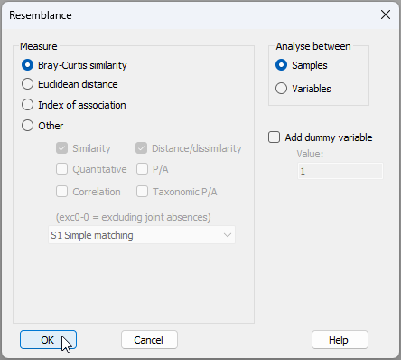
16. From 'Data5', click Analyse > Resemblance... > (Measure $\bullet$ Bray-Curtis similarity) & (Analyse between $\bullet$Samples), 'OK'.

The resulting resemblance matrix will be called 'Resem1', and will look like this:

Ordination via nMDS

17. From the 'Resem1' matrix, click Analyse > MDS > Non-metric MDS (nMDS)..., retain all of the defaults and click 'OK'. The resulting best 2d solution for the nMDS ordination plot is called 'Graph3' in the Explorer tree, and it has a nice low stress of 0.06.

We can consider looking at two different 'views' of this ordination:

• (a) With symbols corresponding to 'Depth' and Labels correspond to 'Latitude' (optionally with trajectories for 'Latitude', split by 'Depth' groups); or
• (b) With symbols corresponding to 'Latitude' and Labels correspond to 'Depth' (optionally with trajectories for 'Depth', split by 'Latitude' groups).

To obtain (a): From 'Graph3', click Graph > Sample Labels & Symbols... (Labels > $\checkmark$Plot > $\checkmark$By factor Latitude) & (Symbols > $\checkmark$Plot > $\checkmark$By factor Depth). Get the trajectories by clicking Graph > Special, click the 'Overlays' tab then choose: Trajectory > $\checkmark$Overlay trajectory > Trajectory numeric factor: Latitude > $\checkmark$Split trajectory Depth.

The result looks like this:

To obtain (b): Simply swap the role of 'Latitude' and 'Depth' factors in the above instructions for (a). The result looks like this:

These ordinations show a very highly spatially structured ecological system, with marked gradual changes in fish assemblages with both latitude and depth. It is clear that latitudinal turnover in fish asesmblages is more marked at shallower depths than at deeper depths. In addition, turnover in fish assemblages with depth becomes less marked after about 600 m, particularly at higher latitudes.

Testing ordered factors via ANOSIM

We can treat each of these factors as ordered factors in a two-way ANOSIM (see Somerfield et al. (2021a) and Somerfield et al. (2021b) ) to test and quantify these effects in a non-parametric (rank-resemblance) framework.

18. From the 'Resem1' matrix, click Analyse > ANOSIM..., and specify the two factors of 'Depth' and 'Latitude' as ordered factors in a two-way crossed design, as shown in the dialog below:

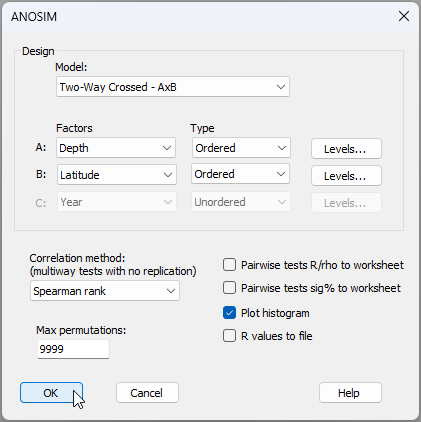
The results (not suprisingly) are uber clear (see the output file 'ANOSIM1' in the Explorer tree). There is a highly significant ordered effect of depth generating sequential turnover in groundfish assemblages from 50 m to 1200 m on the NE Pacific coast (ANOSIM, $R^O$ = 0.934, $P$ = 0.0001). There are also significant sequential changes (i.e., turnover) in groundfish assemblages along the latitudinal gradient, from 32°N to 48°N (ANOSIM, $R^O$ = 0.768, $P$ = 0.0001).

---

^¶NOAA Fisheries, NWFSC/FRAM, 2725 Montlake Blvd. East, Seattle, WA 98112, USA