4.4 Example: Snapper in marine reserves

As an example of the Mann-Whitney U test, we will look at a dataset consisting of counts of the snapper (Chrysophrys auratus) sampled using baited remote underwater videos (BRUVs) from multiple areas inside vs outside several marine reserves along the north-eastern coast of New Zealand ( Smith et al. (2014) ). These data are located in the file ‘NZ_Snapper_counts.pri’, found inside the 'Examples_P8 > NZ_snapper_counts' folder and include the following three variables:

• tot.snapper: Total count of snapper regardless of size (MaxN)
• small.snapper: Count of small snapper $\lt$ 27 cm (MaxN)
• large.snapper: Count of snapper $\ge$ 27 cm (MaxN)

The counts were obtained from video footage as 'MaxN', which is the maximum number of individuals observed in a single frame (during a 60-min period of video, beginning 5 min after the gear makes contact with the sea floor). It is used as an index of relative density. Note also that the minimum legal size for snapper (i.e., the minimum size of fish which may be taken legally by fishers) at the time these data were collected was 27 cm.

There are a number of factors associated with these data. (Click Edit > Factors to see them). Each sampling unit (MaxN value from a given piece of 60-min BRUV footage) is identified by the factor of 'Status' as having been taken from either inside the marine reserve (reserve = 'R') or outside the marine reserve (non-reserve = 'NR'). These are the two groups we wish to compare using the Mann-Whitney U test. Here, we shall focus on comparing reserve vs non-reserve counts of all snapper (tot.snapper) that were obtained only in 2003 and only from the locations of Leigh and Hahei.

Note that, in PRIMER, it is possible to run the Mann-Whitney U test (or any of the univariate non-parametric tests) separately within levels of another factor. In this example, we shall run the test to compare the 2 levels of 'Status' (R vs NR) separately for each 'Location' (Leigh and Hahei). Furthermore, for this example, we shall also (quite naturally) turn to a one-tailed Mann-Whitney U test, as we would expect, a priori, that there would be greater MaxN values recorded from BRUVs deployed inside vs outside any particular reserve at any particular time.

Running the Mann-Whitney U test

1. Open the file ‘NZ_Snapper_counts.pri’ in PRIMER.

2. We may begin by making some simple histogram plots of these count variables. From the 'NZ_Snapper_counts' data sheet inside PRIMER, click Plots > Histogram Plot.... Clearly, the distributions of counts have a very large preponderance of zeros, so the distributions of errors from a classical ANOVA model would not be at all 'normal'. For example, consider the histogram for tot.snapper (shown below):

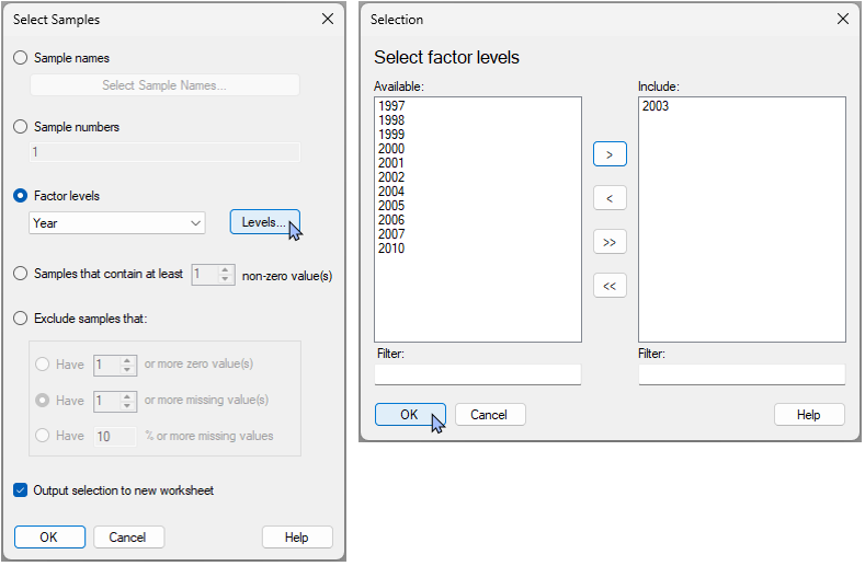
3. Select the 2003 data only. From the data sheet, click Select > Samples... > ($\bullet$ Factor levels: Year > Levels > Include: 2003, 'OK') & ($\checkmark$Output selection to new worksheet).

4. To keep things tidy, you can re-name the resulting sheet (called 'Data1' by default) to '2003_only'. (This is easily done inside the Explorer tree window area, for example):

$\hspace{2cm}$

5. Let’s now do the test. From ‘2003_only’, click Analyse > Univariate > Mann-Whitney…

6. In the resulting Mann-Whitney U Test dialog, choose the following:
   • Variable: tot.snapper
   • Factor: Status
     • Level 1: R
     • Level 2: NR
   • $\checkmark$Within levels of another factor: Location
   • Alternative hypothesis: $\bullet$Level 1 $\gt$ Level 2 (one-tailed)
   • Max permutations: 9999
   • $\checkmark$Output box plot
   • Output values of the test-statistic under permutation: $\checkmark$to graph (histogram)

then click 'OK', as shown below.

Results of the Mann-Whitney U test

The resulting notepad , *.rtf) file named 'Mann-Whitney U test1' contains all of the essential elements of this analysis and its results. First are shown the choices that were made by the user ('Parameters'):

This is followed, in the same output file, by the full suite of results, including all of the relevant supporting calculations ('Results'), viz.:

We can reject the null hypothesis that there are no differences in the total count of snapper inside vs outside the marine reserve at Hahei ($U$ = 175.5, $P$ = 0.0029) and also, even more resoundingly, at Leigh ($U$ = 546.5, $P$ = 0.0001).

Looking next at the graphical output (shown under 'MultiPlot2'), the individual boxplots ('Graph4' and 'Graph6') show these effects and the direction of the differences very clearly: specifically, there was a greater median count of snapper recorded inside the reserve ('R') compared to outside the reserve ('NR') at each of these two locations, viz:

The graphical output also shows histograms of the empirical distributions of the $U^{\pi}$ values (i.e., the values of the test-statistic under permutation) for each of Hahei and Leigh ('Graph5' and 'Graph7', shown below). For this example, we asked for one-tailed tests, so in these distributions, we can see the observed value of $U$ as a dotted vertical line in the upper tail only.

Thus, these marine reserves clearly affected the total counts of snapper obtained from the BRUVs in 2003. Similar comparative tests may be done for different years and/or reserves.

For this example, we might also be interested to compare counts of just the large-sized snapper or just the small snapper, as perhaps the marine reserves only affect distributions of counts for fish that are large enough to be caught (legally) by fishers. We shall leave these ideas for end-users to explore on their own.