9.3 Example: Annual monthly cycles - B.C. macroalgae

Consider the study described by Schenk et al. (2025) consisting of regular surveys of macroalgal cover from a rocky intertidal area at Stanley Park, Vancouver in British Columbia, Canada. Macroalgal communities have been sampled monthly (since September 2021) along each of 3 permanent transects that run from a seawall towards the water, perpendicular to the shore (i.e., from high to low tidal heights). Individual 1 m² quadrats were placed at 5 m intervals along each transect (from 0 to 90 m) and the percentage cover for each of $p$ = 74 macroalgal taxa was recorded.^¶

The full dataset, updated regularly, is available from Borealis. Monthly macroalgal cover data from September 2021 through to April 2025, inclusive, are provided in the file named 'BC_Macroalgal_cover.pri', found inside the 'Examples_P8 > BC_macroalgae' folder. See the file 'BC_Covariables.pri' for associated covariables.

We expect spatial changes in macroalgal assemblages with changes in tidal height, but also cyclically, from month to month, through the calendar year at this temperate latitude (49.3027 $\degree$N). There may also, of course, be changes from year to year. In this example, we shall focus on the temporal factors (year and month) affecting the macroalgal communities at this site. Towards this aim, we will examine a subset of the data, made up of the monthly averages from January 2022 - December 2024 (hence, over three complete years) from quadrats at mid-tidal levels only (specifically, the distance classes from 30 m to 50 m from the seawall, inclusive) and from transects 3 and 4 only, as these have highly similar tidal height profiles. The subsetted and averaged data^§ are held in the file 'Macroalgae_subset.pri' in the 'Examples_P8 > BC_macroalgae' folder.

Set up covariables to code for cyclicity

To test for annual monthly cycles of change in the macroalgal assemblages through these years, we will first need to set up two covariables that code for this cyclicity model, as outlined on the previous page in section 9.2. Steps in the calculation are as follows:

• Let $k$ be the total number of time-points (steps) in the cycle.
• If the time-points, $t = 1, ..., k$, are to be equally spaced, then calculate $c = 2\pi / k$.
• For samples occuring at each time-point $t$ in the cycle, the corresponding values for the two covariables, $x_1$ and $x_2$, are given by:
  • $x_1 = \cos(ct)$; and
  • $x_2 = \sin(ct)$.

The calculations for this example are shown in Table 9.1. The two covariables of 'sin(ct)' and 'cos(ct)', which together code for an annual monthly cycle of change in these macroalgal assemblages are provided in the 'Covariables_subset.pri' data file for this example.

Table. 9.1. Construction of covariables that code for an annual monthly cycle over $k$ = 12 months. For each month ($t$), we have: 'Prop. Dist.' - the proportional/fractional distance around the circumference of the circle (in twelfths) with each succeeding month; 'Dist. Rad' - the distance around the circumference of the circle in radians; and the two covariables that together code for the pattern of cyclicity in 2 dimensions: '$\sin(ct)$' and '$\cos(ct)$', where $c = 2\pi / k$.

Month ($t$)	Prop. Dist. $(t/k)$	Dist. Rad. $(ct)$	$\cos(ct)$	$\sin(ct)$
1	0.08333	0.52360	0.86603	0.5
2	0.16667	1.04720	0.5	0.86603
3	0.25	1.57080	0	1
4	0.33333	2.09440	- 0.5	0.86603
5	0.41667	2.61799	- 0.86603	0.5
6	0.5	3.14159	- 1	0
7	0.58333	3.66519	- 0.86603	- 0.5
8	0.66667	4.18879	- 0.5	- 0.86603
9	0.75	4.71239	0	- 1
10	0.83333	5.23599	0.5	- 0.86603
11	0.91667	5.75959	0.86603	- 0.5
12	1	6.28319	1	0

Note that if some other, possibly unequal, positions along the circumference of the circle are required, each of these can be easily calculated directly from the fractional distances they take along the circumference of the circle. Thus:

• Let $f_t$ be the fractional distance along the circumference of the circle for any given time-point $t$.
• The corresponding values for the two covariables, $x_1$ and $x_2$, at time-point $t$ are then given by:
  • $x_1 = \cos(2\pi f_t)$; and
  • $x_2 = \sin(2\pi f_t)$.

Open the file, transform the data and calculate resemblances

1. Open up PRIMER 8 and click File > Open... to open the data file named 'Macroalgae_subset.pri' (found inside the 'Examples_P8 > BC_macroalgae' folder).

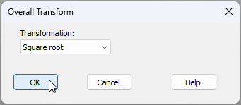
2. From the 'Macroalgae_subset' data sheet, click Pre-treatment > Transform(overall)..., choose 'Square root' from the drop-down menu, then click 'OK'.^†

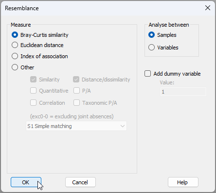
3. This will yield a data sheet of square-root transformed values called 'Data1'. From this, calculate Bray-Curtis similarities among the samples by clicking Analyse > Resemblance... and going ahead with the defaults in the resemblance dialog (as shown below) by clicking 'OK'.

The result will be a resemblance matrix among the samples, called 'Resem1', as shown below:

Create an ordination with temporal trajectories

We wish to visualise these relationships among the sampling units, which may be achieved using ordination via non-metric MDS. More specifically, we hope to visualise how macroalgal assemblages may change from month to month and/or from year to year. We wish, in particular, to discern whether a cyclical pattern of change in macroalgal assemblage structure is evident through each calendar year on our ordination plot, so a trajectory that connects the sequentially ordered months through each year would be helpful here.

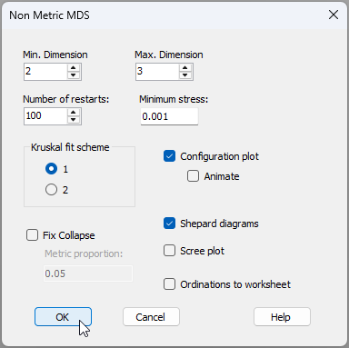
4. From the 'Resem1' matrix, click Analyse > MDS > Non-metric MDS (nMDS)..., go with the defaults in the 'Non Metric MDS' dialog, but choose 'Number of restarts: 100' (as shown below), then click 'OK'.

5. The lowest stress 2D nMDS that could be achieved by the algorithm will be provided in an item called 'Graph1' in the Explorer tree (as part of the 'MultiPlot1' output). It should look like this:^‡

Let's now take two simple steps to make this graphic easier to interpret by reference to our temporal factors of interest.

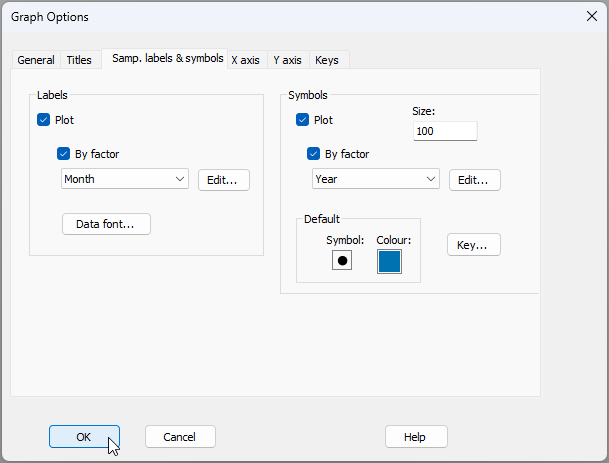
6. First, let's change the labels on the points to show the months. From 'Graph1', click Graph > Sample Labels & Symbols..., then choose to plot the 'Labels' $\checkmark$By factor Month, (and leave it so that the Symbols are plotted $\checkmark$By factor Year), precisely as shown in the dialog below, then click OK.

7. Second, let's overlay a trajectory through the consecutive months within each calendar year. From 'Graph1', click Graph > Special.... Click on the 'Overlays' tab, then choose to $\checkmark$Overlay trajectory by the numeric factor of Month. Choose also to $\checkmark$Split trajectory by Year, and untick the box in front of the words '$\Box$Add arrow heads and tails', as shown in the dialog below:

The resulting nMDS plot will now look like the image below, which is much easier to interpret.

In each year, we can see a clear pattern of cyclical change in these macroalgal assemblages, from months 1 through 12. The greatest changes in assemblages appeared to occur in the early months of 2022 (months 1-4 for the amber symbols, from left to right in the plot), but the annual cycles of monthly change that occured in subsequent years (2023 and 2024, in green and blue) were broadly similar in both size and direction.

Create the PERMANOVA design file

Having seen these patterns, we are naturally keen now to perform a formal test of cyclicity. To do this, we need to bring in the covariables for these data and create an appropriate design file to run the PERMANOVA. This is where we will implement the new feature in PERMANOVA to group covariables together, as our cyclical model requires the simultaneous action of two covariables in order to adequately capture this two-dimensional pattern in the multivariate response.

8. Bring in the file containing the relevant temporal covariables that are associated with the subsetted and averaged dataset. Click File > Open... and open the data file named 'Covariables_subset.pri' (found inside the 'Examples_P8 > BC_macroalgae' folder).

From the 'Covariables_subset' sheet now in the Explorer tree, click Edit > Indicators... and you will see that there is an indicator called 'Cov.group' for this dataset, showing that both of the variables 'sin(ct)' and 'cos(ct)' belong to a single group called 'Annual.monthly.cycle'.

9. From the 'Resem1' resemblance matrix, click PERMANOVA+ > Create PERMANOVA design..., then do the following:

• Double-click the first blank cell (under the word 'Factor'), and choose the factor of 'Year' from the drop-down menu so that it shows in the first cell (row 1, column 1) of the design file. Also, specify that the 'Type' of this factor is 'Random' (double-click the cell in row 1 column 3 to bring up that dialog).

• Next, in the section of the dialog entitled 'Covariables', use the drop-down menu to choose the 'Worksheet:' as 'Covariables_subset', then tick the box to $\checkmark$Group covariables (indicator) and choose the indicator 'Cov.group' for this, as shown below:

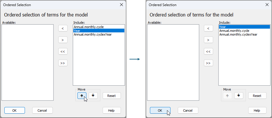
If you now click on the 'Terms' button () under the words 'Sources of variation' in this design file, you will see that the terms in the model include 'Year', 'Annual.monthly.cycle', and their interaction. Notice that the default in PERMANOVA is to put the covariable(s) first. For this analysis, however, it might seem somewhat more natural to fit 'Year' first, as the largest temporal scale. To order the terms in this way, click on the word 'Year' inside the 'Include:' box and then on the upwards arrow under the word 'Move' in the dialog, then click 'OK', as shown below.

Now we are ready to run the PERMANOVA model on the basis of this finalised design file.

Run the PERMANOVA analysis

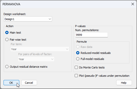
10. From the 'Resem1' matrix, click PERMANOVA+ > PERMANOVA.... Ensure that the correct design worksheet file is nominated here ('Design1'), keep all of the other defaults, as shown below, then click 'OK'.

The PERMANOVA output file and table of results are very clear. The annual monthly cycle is a term with 2 degrees of freedom, and this is highly statistically significant ($F_{2,25}$ = 14.491, $P$ = 0.0001). There are also significant differences among the three years ($F_{2,25}$ = 3.8407, $P$ = 0.0001), but the sizes of yearly effects are not as large as the effects of monthly seasonal changes within each year (cf. the sizes of their respective estimated components of variation). Interestingly, there is also a significant interaction term ($F_{4,25}$ = 1.5997, $P$ = 0.0465), indicating that the nature of the monthly cycles differs somewhat among the years. These results align well with the earlier patterns seen in the nMDS ordination; specifically, clear cyclical patterns and also some deviations in the size of the cyclical pattern for 2022 compared to the other two years.

---

^§There were no data available from transects 3 and 4 at these mid-tidal levels (30 m - 50 m distances) in September 2022 and in October 2023, due to the tide not being sufficiently low on the dates of sampling, so these two data points are missing from this example.

---

^¶ If the estimated percentage cover was between 0% and 5%, then a percentage cover value was estimated to the nearest 1%. If the estimated percent cover was over 5%, then percentage cover was estimated to the nearest 5%. Therefore, the cover values were: 0, 1, 2, 3, 4, 5, 10, 15, 20, ..., 95, 100. Note also that the total percentage cover measured within a single quadrat could exceed 100%, due to there being multiple layers of different species of macroalgae.

---

^† The square-root transformation is typically a good one to use when dealing with percentage cover data, as the raw values tend to range from 0 to ~100 percent, hence the square-root values will tend to range from 0 to 10. This places different taxa on a fairly even footing, yet retains information regarding differences in relative percentage cover values.

---

^‡You may find that your particular nMDS solution has the same stress, but is 'reflected' across the X and/or Y axes. From 'Graph1, you can click Graph > Flip X and/or Graph > Flip Y in order to check this and (optionally) change it.