7.2 Dichotomy: fixed vs random factors
Consider the classical one-way linear ANOVA model, as described in section 6.2 above. Specifically, we have a random variable $Y$, and we have taken a sample of size $n_i$ from each of $i = 1,\ldots, a$ groups to obtain observed values $y_{ij}$. Thus, factor A has $a$ groups or levels. We can visualise the ANOVA model graphically as shown in Fig. 7.1.
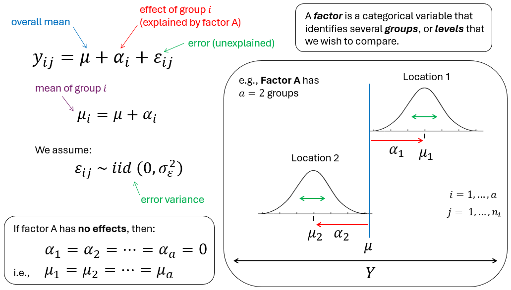
Fig. 7.1. A schematic diagram of the ANOVA linear model.
Specifically, we can imagine (in the univariate case) that $Y$ is represented on a number line going from left to right. To arrive at any particular value $y_{ij}$, we begin at the overall mean, $\mu$. To this we add the effect of being in a particular group, $\alpha_i$. If the effect is non-zero it will shift us (up or down) along the number line a distance of $\alpha_i$ away from the overall mean, $\mu$, to arrive at the position $\mu_i$, which is the mean for group $i$. To arrive at the value equal to our particular observation $y_{ij}$, we must then also add the error, $\varepsilon_{ij}$ associated with that individual observation.
What do we assume about the overall mean, the effects and the errors?
- For the overall mean, we (classically) assume that it is a fixed unknown constant.
- For the errors, we assume that they are each drawn randomly and independently from an (effectively) infinite population distribution that has a mean of zero and a variance of $\sigma_\varepsilon^2$.
- What we assume about the effects depends on whether factor A is fixed or random.
- If factor A is fixed, then the effects, $\alpha_i$, are considered to be fixed unknown constants (like $\mu$).
- If factor A is random, then the effects, $\alpha_i$, are considered each to have been drawn randomly and independently from an (effectively) infinite population distribution that has a mean of zero and a variance of $\sigma_\alpha^2$.
The criteria that are typically used in order to decide whether an individual factor is fixed or random are given in the Table below.
Table 7.1. Criteria for identifying a given factor as either fixed or random.
| Fixed factor | Random factor |
|---|---|
| The effects, $\alpha_i$, are fixed unknown constants. There is a finite number of levels, and all of them (or all of them of interest) occur in the study. | The effects, $\alpha_i$, are a subset of levels drawn from an infinite (or uncountably large) population of possible levels. |
| If we were to repeat the study, the same levels would be chosen. | If we were to repeat the study, the same levels might not be chosen. |
| Interest lies in the individual effects, $\alpha_i$. | Interest lies in the variance component, $\sigma_\alpha^2$. |
| We will want to do pair-wise comparisons for this factor, if the factor is significant. | We are typically not interested in pair-wise comparisons for this factor. |
| H0: $\alpha_1 = \alpha_2 = \ldots = \alpha_a = 0$ | H0: $\sigma_\alpha^2 = 0$ |
| Inferences are about only the specific levels of the factor included in our study. | Inferences are about the whole population of possible levels for that factor that we could have sampled. |
Examples of fixed factors could be:
- Habitat: {seagrass, kelp forest, rocky reef}
- Maturity: {adult, juvenile}
- Treatments: {high-dose, low-dose, placebo, control}
- Status: {pristine, restored, disturbed}
In each of the above examples, we can see that the names of the levels have a particular meaning in the context of the experiment or sampling design. These levels are not a random sample of possible levels. In each case, they correspond to something specific that we have chosen a priori to investigate. We would definitely like to know, for example, what the effect is of (say) the low-dose treatment compared to that of the high-dose treatment, if any. If the levels of the factor have specific names or labels like this, then this is a direct indication that the factor is fixed; the researcher cares about the levels themselves, and has set up the sampling design or experiment to measure and understand these particular effects. We would (almost certainly) be keen to follow-up any significant $F$-ratio with subsequent pair-wise comparison tests to examine how the individual levels might differ from one another.
Even if the levels included in the study do not correspond to 'all possible levels' of a given factor, there is still a clear sense that the levels of a fixed factor that are included in the study correspond to all those that are of interest. For example, suppose we design an experiment to investigate the effect of temperature on the growth of an organism, and have set up a series of (replicated) microcosms at each of three different levels: {20$^{\circ}$C, 23$^{\circ}$C, and 26$^{\circ}$C}. Clearly, we have not sampled all possible temperatures. Nevertheless, these are the only temperatures about which we intend to make inferences, and we would therefore treat 'Temperature' as a fixed effect.
Examples of random factors could be:
- Batches: {B1, B2, B3, ...}
- Transects: {T1, T2, T3, ...}
- Sites: {S1, S2, S3, ...}
- Years: {Y1, Y2, Y3, ...}
For random factors, typically the levels are not, individually, of any particular interest. A random factor might be included in a study purely for logistic reasons. For example, suppose you are studying the behavioural response of soldier crabs to human by-standers. It may not be feasible to get sufficient replication of your experimental protocols in the field all at once, simultaneously, so you might have to run your study in batches over a period of days. Thus, 'Batch' (and/or 'Day') then becomes a random factor that contributes a potential source of variation to your results.
In other cases, random factors occur because interest lies precisely in measuring variability at one or more spatial or temporal scales. For example, we might expect variation in the abundance of settlers for organisms that are brooders to be higher than that of broadcast spawners in marine environments at large spatial scales. Settlers of each type of organism (brooders and spawners) can be monitored at a series of sites (separated by, say, hundreds of metres), and the factor of 'Sites' would be a random factor. There may be a very large number of sites that we could have sampled, but we will likely be able to sample only a very tiny fraction of these as a subset (suppose we sample 10 sites). Measuring the abundance of settlers in replicate quadrats at each of the $a$ = 10 sites, we care not at all how the mean may differ between (say) site 3 and site 8; pair-wise comparisons are of no interest. We do wish to examine if site-to-site variation is detectable over-and-above residual variation (hence, to test H0: $\sigma_\alpha^2 = 0$), and, if so, to estimate the size of $\sigma_\alpha^2$ separately for brooders and spawners.
Importantly, whenever we set up an experimental/sampling design (e.g., in a'Design' file in PERMANOVA for PRIMER), the choices that are made in this regard (for each factor) will have very important consequences for:
- the assumptions underlying the PERM(ANOVA) model;
- the expected values of mean squares (EMS) for each term in the model;
- the construction of an appropriate $F$ ratio for individual terms in the model;
- the construction of an appropriate permutation algorithm (under exchangeability);
- the hypothesis being tested by the $F$ ratio; and
- the extent and the nature of the statistical inferences.