7.3 Not a dichotomy: a progression from fixed to random

What is meant by a 'finite' factor?

Suppose, for any factor, there are a total of $A$ levels in the population. In some cases, $A$ is absolutely enormous and it may be effectively infinite in the sense of being uncountable (e.g., blades of seagrass in a large seagrass meadow). In other cases, $A$ might well be finite (e.g., there might only be a total of $A$ = 10 restored areas).

In any given study, the researcher may sample (i.e., randomly and representatively draw, without replacement) $a$ levels out of the $A$ total possible levels for any given factor. The sampling fraction is therefore $a/A$. The larger the sampling fraction, the more the researcher will know about the system, hence, the greater the potential power in drawing inferences from the study about that factor.

Now, a fixed factor occurs where all possible levels are drawn, so $a=A$ and the sampling fraction is $a/A = 1$. The finiteness of fixed factors is quite clear. For example, the levels 'treatment' and 'control' do not come from a wider population: together they comprise a 'population' of only 2 levels. These are naturally the only two levels of interest in the study and $a = A$ = 2.

On the other hand, a random factor occurs where $A$ is extremely large (effectively infinite), and hence our sampling fraction $a/A$ is very tiny (approaching zero in the limit).

A progression of steps from fixed to random

It is quite easy to conceive, however, of a finite population of levels where $A$ is known, but we cannot sample all possible levels, and $A > a$. For example, suppose I am able to sample $a$ = 4 restored habitats (islands) out of a total of $A$ = 10 restored habitats that occur in a given region of interest. In this case, the sampling fraction is $a/A$ = 4/10 = 2/5. This fraction is neither trivially small (random), yet nor is it precisely equal to 1 (fixed). In this way, more generally, we can see that there is an incremental progression of steps, from fixed to random, that depends on the sampling fraction (Fig. 7.2).

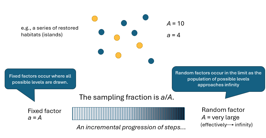
Fig. 7.2. A series of steps in the progression from fixed to random factors.

The finiteness of the population of possible levels will tend to become more apparent (and more important) as the spatial or temporal scale of the factor gets larger. For example, suppose I repeat an experiment on the effects of fish predators at each of three separate bays along a coastline. I may well wish to include the factor of 'Embayment' in my study design. What are these three embayments intended to represent? Are there many such embayments, or only a handful? Have I sampled all of them or a substantial fraction of them? These are important questions to answer so as to ensure we achieve maximum power to test relevant hypotheses in our study.

Statistical derivations of EMS

Cornfield & Tukey (1956) articulated the concept of the experimenter sampling levels of factors from finite vs infinite populations, and they showed the resulting outcomes for expectations of mean squares (EMS), and therefore how to construct correct $F$ tests, in two-way and three-way crossed balanced designs for univariate ANOVA cases.

Anderson et al. (2025) combined these results with the landmark work by Hartley (1967) , Rao (1968) and Hartley et al. (1978) for balanced and unbalanced cases, thereby incorporating the sampling fraction from finite populations into the derivation of EMS by 'synthesis' for any general complex ANOVA design. Anderson et al. (2025) further extended these results to multivariate dissimilarity-based tests using PERMANOVA. The new PERMANOVA routine in PRIMER 8 fully implements the methodology described by Anderson et al. (2025) , with correct tests constructed by reference to the EMS via 'synthesis'. Specifically, the new PERMANOVA routine in PRIMER 8 permits:

• any individual factor to be specified as 'fixed', 'random' or 'finite' (a new factor type);
• the size(s) of any finite populations (i.e., the total number of levels) to be specified for each finite factor;
• finite factors in asymmetrical designs (e.g., where there may be different numbers of levels in different parts of the study design, such as 1 impact location and multiple controls).

Motivation

Motivation for the development of an option to fit finite factors in PERMANOVA arises especially in the context of ecological studies of environmental impact. We wish generally to permit flexibility in the definitions of factors where the sampling fraction is neither equal to 1, nor infinitely small. Studies of environmental impact will often contrast responses of organisms measured at a purportedly impacted location vs one or more 'control' (reference or unimpacted) locations ( Underwood (1991) , Underwood (1992) ). In such a design, one views the control locations as being a random sample from some larger population of control locations that are (apart from the impact itself) environmentally similar to the impacted location ( Underwood (1994) , Glasby (1997) ). It is desirable to sample as many control locations as logistics/time/funding will permit, so as to increase both the power of the test and the scope of the inferences ( Glasby (1997) , Glasby & Underwood (1998) ). In practice, however, the population of possible control locations is likely to be both finite and limiting, particularly at large spatial scales. In such cases, we might consider the (single) impacted location as being 'fixed' (e.g., a single oil spill, a single sewage outfall, a single storm, etc.), while the reference locations can be treated as either random or drawn from a finite population of a specified size.

Next, we shall provide an example of a PERMANOVA analysis involving a finite factor in the context of a study of the potential environmental impact of a sewage outfall on mollusc assemblages inhabiting rocky subtidal habitats on the coast of Italy (Mediterranean Sea).