14.1 Overview
There is a new tool in PRIMER 8 that permits the end-user to create a set of ordered groups, based on the numerical values of a given variable.
Rationale
Below we provide a few examples of this tool's potential utility. There are many more!
Binning and consolidating information
A case where we might want 'categories', but where there may be (initially) continuous values, occurs when we have a broad-scale dataset with a lot of replicates that span a very large area or domain (in terms of latitude and longitude). For example, consider the Continuous Plankton Recorder (CPR Survey. Many other ocenographic, landscape-level and environmental datasets have these characteristics. We might want to consolidate that information in some way, perhaps in order to make comparisons with more discrete (less continuous) datasets or variables (e.g., dis-continuous biotic samples at particular sites or regions). We could consider making a 'grid' over the sampling extent (i.e., by creating 1-degree sized bins for each of latitude and longitude) and then get the average values of the variable(s) within those grid cells. Indeed, to understand spatial relationships and patterns, it may be essential to bin samples into latitude (and/or longitude) groupings, so that structural changes through space can be more easily summarised, tested, visualised in plots, etc.
Classification based on an ordination axis
Let's consider another scenario. Perhaps you have just done a principal component analysis (PCA) on a set of morphometric variables (e.g., for a set of individuals belonging to a given species). Suppose the first PC axis explains a lot of the multivariate variation and the position of any individual on that PC axis can essentially be interpreted as a measure of its overall relative size. The values of the individuals on the PC axis are continuous, but maybe you want to classify the individuals into (say) five roughly equal-sized groups along that axis (from small to large). In the past, this task could have taken some considerable time, sorting and data wrangling to get your groups based on the PC axis. Our new tool in PRIMER 8 will create equal sample-sized groups along your chosen continuous variable (e.g., a PC axis, or any other meaningful ordination axis of choice) in a flash.
Setting known break points in the data
Yet another use-case for this tool is the situation where you want to identify a set of samples that fall within a certain range of values for a continuous variable; for example, suppose you want to separate out samples occuring at sites that are below a certain temperature (e.g., 20°C). You can use the tool to specify the value of 20 as a 'break point', and get a factor that groups samples either side of that break point. Multiple such breaks points can also, optionally, be constructed all at once. For example, suppose you have the continuous variable of depth (in metres); you might want to 'bin' samples into several categories according to their depths, using break points of 10, 20, 30, 40, etc. (We shall see an example of this in the next section.)
Finding natural peaks or gaps to define groupings
You may have a continuous variable that is not evenly distributed across its full range. For example, a histogram may show a multimodal distribution pattern. You may want to define groups that coincide in some natural way with that uneven distribution, such that each group will capture an individual 'mode' or 'peak'. You may not be certain about where the break-points in-between those modes should be placed. In this case, you would want the tool to find suitable break points for you by (say) minimising the within-group sum of squares for the variable, given the number of groups (peaks). If the modes are asymmetric, then sums of distances-to-median (rather than the within-group sum of squares) might be more appropriate to use here. Or you could go even more non-parametric in your criterion and choose groups so as to minimise only the rank inter-point Euclidean distances within each group.
Specifying groups of replicates for dispersion weighting
Many species abundance variables (e.g., counts) display intrinsic mean-variance relationships. In other words, the variance increases with the mean. This relationship is particularly strong and important to consider in the context of species that tend to aggregate, e.g., such as fish that school, birds that flock, mammals that travel in herds, insects that cluster together in swarms, etc. We may wish to accommodate this by applying a pre-treatment to our data called dispersion weighting (see Clarke et al. (2006a) for details). This pre-treatment option effectively transforms our data to consider the abundances (counts) of clusters of organisms (for those species that do indeed demonstrate significant clustering of individuals), rather than analysing the raw abundance values. Of course, the dispersion weights that may be needed here will vary according to the individual species' distribution of counts across the sampling units.
To characterise mean-variance relationships, hence to apply dispersion-weighting, we need groups (levels of some factor) across which we can calculate and measure means and variances. In cases where we do not have any groups to begin with (e.g., whenever our sampling units occur along a continuous gradient, in a simple spatial array or regular samples through time, etc.), then there will be no way to use dispersion weighting at all. Usnig this new tool, we can create groups along one (or more) continuous variables which can then form the basis of a dispersion-weighting pre-treatment option.
Plotting symbols and colours
It can be extremely useful to create groups from a continuous variable for rather simple practical or logistic reasons. For example, suppose we want to use different colours or symbols for different levels of a continuous variable, such as temperature. We may not want to have a different colour for every single temperature, but rather we might prefer to have a colour (and/or symbol) for all cases where temperature values occur within some specified range, for each of a set of specified temperature groups (eg., low, medium and high). The use of well-defined symbols and colours like this can make interpretations of patterns in ordinations, especially along gradients, much easier to visualise and communicate to others.
Implementation
This tool is accessed by clicking Tools > Create Ordered Groups.... The dialog window is shown below.
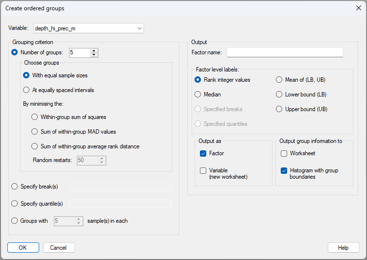
There is clearly a large diversity of options to choose from to create ordered groups based on a chosen continuous variable, as shown in the dialog above. The various methods that can be used to create groups are itemised and outlined, correspondingly, in more detail below.
Methods for creating groups
Consider an individual variable $Y$, which has a set of observed sample values $y$ and which our algorithm is going to split into $g$ ordered groups using some criterion. Let the number of sample values in each group be denoted by $n_i$ for $i = 1, \ldots, g$ and the total number of sample values is $\sum_i^g n_i = N$. Also, let $y_{ij}$ denote the $j$th observed value of $Y$ in the $i$th group for $j = 1, \ldots, n_i$ and $i = 1, \ldots, g$. In what follows, we shall let $\bar{y}_ i = \sum_{j=1}^{n_i} {y_{ij}} / {n_i} $ be the sample average of the variable for group $i$, and $m_i$ be the median value for the set of samples in group $i$.
The methods for choosing ordered groups based on the variable $Y$ include:
- (1). Specify the number of groups, $g$, and, given that number, generate groups:
- (a). with equal sample sizes ($n_1 = n_2 = \cdots = n_g$); or
- (b). at equally spaced intervals, so as to minimise:
- (i). the within-group sum of squares, i.e., $\sum_{i=1}^{g}\sum_{j=1}^{n_i} (y_{ij} - \bar{y}_ i)^2$; or
- (ii). the sum of within-group mean absolute deviations (MAD) from the median, i.e., $\sum_{i=1}^{g}\sum_{j=1}^{n_i} |y_{ij} - m_i|$; or
- (iii). the sum of within-group average rank inter-point Euclidean distances.
- (i). the within-group sum of squares, i.e., $\sum_{i=1}^{g}\sum_{j=1}^{n_i} (y_{ij} - \bar{y}_ i)^2$; or
- (a). with equal sample sizes ($n_1 = n_2 = \cdots = n_g$); or
- (2). Specify break(s) manually, i.e., a list of specific values of the variable that will serve as break-points between consecutive ordered groups (e.g., 10, 20, 50, 100); or
- (3). Specify the quantile(s) of the variable's empirical distribution where you want break-points to be (e.g., 0.25, 0.5, 0.75); or
- (4). Specify groups by nominating a certain value for the number of samples in each group, i.e. $n_i = n$ for all $i$.¶
†Dispersion weighting ( Clarke et al. (2006a) ) is achieved easily and directly in PRIMER 8 by clicking Pre-treatment > Dispersion Weighting....
¶Note that if there are any 'remainders', given the total sample size, these will be placed in a final group, corresponding to the largest values of the variable, but with reduced $n$. For example, if you have 10 samples and you ask for groups having a sample size of $n$ = 3, the tool will create 3 ordered groups {1,2,3}, {4,5,6}, {7,8,9}, and one remainder sample will spill into a fourth group on its own {10}.