8.2 Example: Split-plot - Woodstock vegetation

The study design

An example of a split-plot design is provided by a study of the effect of fire disturbance and grazers (excluded using fences) on the composition of plant assemblages on the central western slopes of New South Wales in south-eastern Australia ( Prober et al. (2007) ). The design (shown schematically in Fig. 8.4) included the following:

• Blocks (random with $r$ = 4 levels).
• Factor A: Fire frequency (fixed with $a$ = 4 levels: 0 yrs, 2 yrs, 4 yrs, or 8 yrs).
• Whole plots (random and nested within Blocks and Fire frequency, unreplicated).
• Factor B: Fencing (fixed with $b$ = 2 levels: fenced or unfenced).
• Sub-plots (random and nested within all of the above, unreplicated).

The two fencing treatments were randomly allocated to two sub-plots (measuring 5 m $\times$ 5 m) within each fire treatment (whole plots) and there is one of each fire treatment (4 whole plots) randomised within each block. Relative abundances (cover) of higher plant species within each sub-plot were estimated using a point-intercept technique (an 8 mm dowel placed vertically at each of 50 points on a grid across each plot). Although the design was set up at each of two locations (Woodstock and Monteagle) and data were obtained over a number of years (see Prober et al. (2007) for more details), we consider here only data from the Woodstock location collected in 2003.

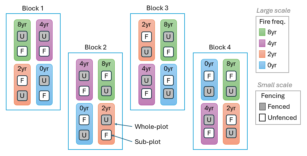
Fig. 8.4. Schematic diagram of the Woodstock split-plot design examining the potential effects of fire frequency and grazers (excluded using fences) on plant assemblages.

For the multivariate analysis, we also will exclude two species from the plant assemblage: Poa sieberiana (grey tussock grass) and Themeda australis (kangaroo grass), both dominant grasses, from the analysis. These were analysed separately in detail by Prober et al. (2007) ; our focus here instead will be on the more subtle potential responses of subsidiary forbs and exotic species.

Input data and select variables

1. Start running PRIMER 8, then click File > Open... to open the data file named 'Woodstock_grassland.pri' (found inside the 'Examples_P8 > Woodstock_grassland' folder).

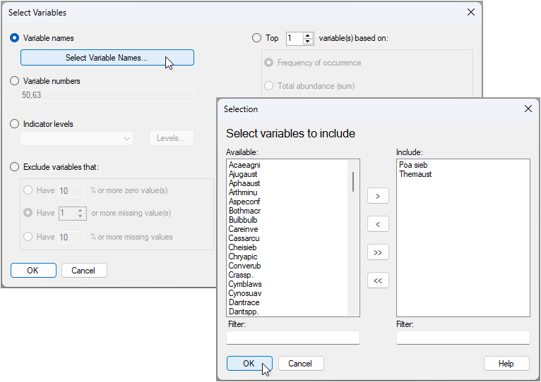
We want to select all variables except the two dominant grasses. We will first find these two variables in the data file, highlight them and then invert that highlighting in order to select the remaining species. The two dominant grasses Poa sieberiana and Themeda australis are named 'Poa sieb' and 'Themaus' in the data file, respectively.

2. Click Select > Variables... > ($\bullet$ Variable names), then click on the button 'Select Variable Names...'. In the resulting dialog, start typing 'Poa' in the 'Filter:' box under the 'Available' box on the left. When you find 'Poa sieb', you can click on its name, then click the right arrow to move this over to the 'Include' box on the right. Repeat the same operation to find and include 'Themaus'. Once both variables you want to select are in the 'Include' box, click 'OK', then click 'OK' in the 'Select Variables' dialog window.

The data sheet with only these 2 species selected will look blue in colour, like this:

3. From the data sheet having only these 2 species selected, perform the following steps:
   • click Select > All. This will show the full spreadsheet of all species once again, but now those two species will just be highlighted (appearing in orange / pale yellow) within the sheet.
   • click Edit > Invert Highlight. Now all of the species except 'Poa' and 'Themaus' (and all of the rows) will be highlighted.
   • click Select > Highlighted. Now all of the species except 'Poa' and 'Themaus' will be selected (hence blue).
   • click Tools > Duplicate, to produce a new separate data sheet (which now omits those two grass species) called 'Data1'.

Calculate the resemblance matrix

For analysis of composition of the assemblage, we will apply a square-root transformation, followed by the Bray-Curtis resemblance measure.

4. From the 'Data1' data sheet, click Pre-treatment > Transform(overall)... and choose 'Square root' from the drop-down menu, then click OK. This will generate a new data sheet item containing the transformed data, called 'Data2'.

5. From the square-root transformed data ('Data2'), click Analyse > Resemblance... and in the 'Resemblance' dialog window, choose (Measure: $\bullet$Bray-Curtis similarity) and (Analyse between: $\bullet$Samples), then click 'OK'. This will yield a resemblance matrix item in the explorer tree, called 'Resem1'.

Create the design file

Recall that running a PERMANOVA will require us first to set up a design file in accordance with our study's experimental/sampling design.

6. From the 'Resem1' matrix, click PERMANOVA+ > Create PERMANOVA Design..., then, in the resulting design file (called 'Design1'), click three times on the button to add a row () so that there are four rows in total, as shown below.

7. Choose the name of the factor you want in each row - In this design file (called 'Design1'), double-click inside each cell of the first column (headed 'Factor') in order to choose the following factors so that they occur sequentially in rows 1, 2, 3 and 4, respectively: row 1 = 'Block', row 2 = 'Fire frequency', row 3 = 'WholePlot', and row 4 = 'Fencing', as shown below:

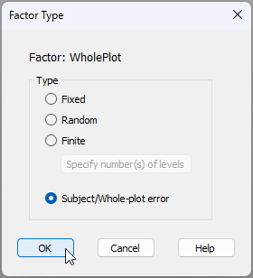
8. Input the factor types - Next, in column 3, we need to specify the 'Type' of each factor. By default, everything begins by being listed as 'Fixed'. To change this for any given factor, we double-click on the word 'Fixed' in its respective row and the 'Factor Type' dialog will pop up. For the present design, we are happy to treat the factors of 'Fire frequency' and 'Fencing' as 'Fixed', but we need to specify carefully that:
   • 'Block' is of Type '$\bullet$ Random', and
   • 'WholePlot' is of Type '$\bullet$ Subject/Whole-plot error', like so:

Having done that, the final correct design file (called 'Design1') for this split-plot study will look like this:

Further design considerations

Before we run the analysis, it is worth pointing out a couple of things about this design file.

First, you will notice that there is a dash ('-') in the 'Nested in' column for the factor of 'WholePlot'. This is because whole-plots, having been identified as such, are deemed effectively to contribute an 'error' into the study design, which means they are necessarily nested within all of the broad-scale factors (in the present case, the broad-scale factors are 'Block' and 'Fire frequency'). Having specified that 'WholePlots' are of Type 'Subject/Whole-plot error', it is not necessary to also articulate this nested structure as well. The dash ('-') merely indicates this column has been 'taken care of' internally, so-to-speak, for the whole-plot factor.

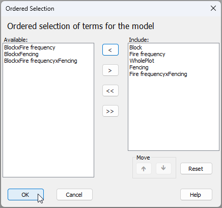
Second, if you click on the 'Terms...' button (), you will see (on the right-hand side, in a box under the word 'Include:') a list of all of the terms included (by default) in the full PERMANOVA model implied by the design that you have specified.^¶ In the present case, it looks like this:

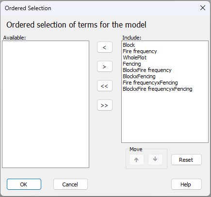
What do we know about this design already?

• (i). The 'Block$\times$Fire frequency' interaction term is not actually estimable, because there is no replication of the Fire-frequency treatments in each block.
• (ii). The 'Block$\times$Fire frequency$\times$Fencing' interaction term is also inestimable, because there is no replication of the two fencing treatments in each whole-plot.
• (iii). The 'Block$\times$Fencing' interaction term would not typically be included in a classical analysis of a split-plot design like this. This is primarily because blocks are set up at large scales and the fencing treatment is applied at small scales.

It turns out that, classically, none of the interactions involving the factor of 'Block' would be included in the ANOVA partitioning for this split-plot design. The sources of variation and degrees of freedom for this example, according to a traditional split-plot ANOVA partitioning, are shown in Table 8.1

Table 8.1. Sources of variation and degrees of freedom ($\textit{df}$) for a classical split-plot design, where factor A = 'Fire frequency' and factor B = 'Fencing', as per the Woodstock example. Note that 'Whole-plot total' is not an additional source of variation, but rather corresponds to the total variation at the broad scale, i.e., among all of the whole plots, which may be relevant for terms in the top half of the table only. (The line corresponding to 'Whole-plot total' can simply be omitted).

Source	$\textit{df}$
Block	$(r-1) = 3$
Fire frequency	$(a-1)=3$
Whole-plot error	$(r-1)(a-1) = 9$
Whole-plot total	$(ra-1) = 15$
----------------------------------------	------------------------------------
Fencing	$(b-1) = 1$
Fire frequency$\times$Fencing	$(a-1)(b-1) = 3$
Sub-plot error	$a(b-1)(r-1) = 12$
Total	$abr - 1 = 31$

If we run the PERMANOVA directly, without manually removing any of the interactions involving the factor of 'Block', then both (i) 'Block$\times$Fire frequency' and (ii) 'Block$\times$Fire frequency$\times$Fencing' interaction terms will be removed automatically in the PERMANOVA run anyway, as these two terms are inestimable. However (in this example), the (iii) 'Block$\times$Fencing' interaction term will remain in the model, simply because it is (technically) estimable.

9. Remove unwanted interaction terms (optional) - If you desire the classical split-plot design, you may wish to manually remove all of the interaction terms involving the factor of 'Block'.^‡ To do this, click on the 'Terms' button in the design file and (sequentially) click on each of the terms that you wish to omit from the model, then click on the left arrow () to move it over to the 'Available' column. The result (if you do choose to remove all of the interactions involving the factor of 'Block') will look like this:

Click 'OK' and now the design file is all ready for the split-plot analysis.

Run the PERMANOVA

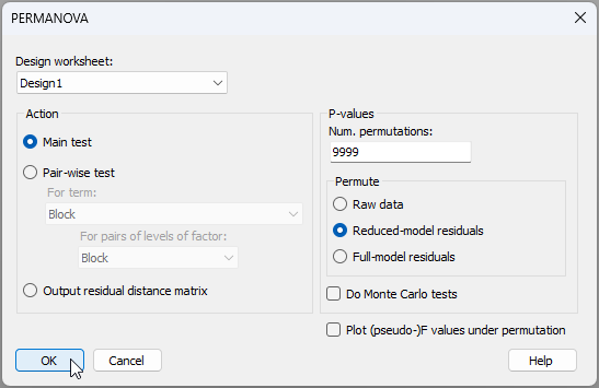
10. From the original resemblance matrix 'Resem1', click PERMANOVA+ > PERMANOVA.... Ensure that the design worksheet is 'Design1', leave all other defaults, and click 'OK'.

The resulting output file (called 'PERMANOVA1') looks like this:

There is a significant effect of fire frequency on the composition of these plant assemblages ($F_{3,9}$ = 2.08, $P$ < 0.01). There was not, however, a significant effect of fencing to exclude grazers ($F_{1,12}$ = 1.45, $P$ > 0.10), nor did fencing treatments change the overall effect of fire frequency (the Fire frequency$\times$Fencing interaction term was not significant; $F_{3,12}$ = 1.29, $P$ > 0.10).

Run pair-wise comparisons

A natural next step might be to examine pairwise comparisons among the whole-plots having different fire frequencies.

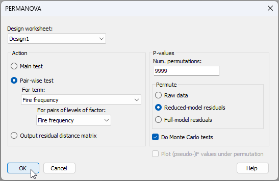
11. To run pairwise tests, start from the original resemblance matrix ('Resem1') and click PERMANOVA+ > PERMANOVA.... Ensuring, once again, that the design worksheet is 'Design1', under 'Action', choose: ($\bullet$Pair-wise test > (For term: Fire frequency > (For pairs of levels of factor: Fire frequency) ) ). You might also (optionally) tick the option to '$\checkmark$Do Monte Carlo tests', simply because there are not very many whole plots to permute at the large spatial scale. Leaving everything else as the defaults, click 'OK', viz:

Results of the pairwise comparisons are shown below ('PERMANOVA2'):

Despite the significant overall test, individual treatment levels are not detected as being significantly different from one another (at the 0.05 significance level) in the pair-wise tests.^† This sort of thing can happen, as the overall (omnibus) $F$-test can have greater power, given its larger denominator degrees of freedom, compared to the individual pair-wise tests.

Ordination of whole-plot centroids

Given that fire frequency is assessed at the spatial scale of entire whole-plots (and fencing had no detectable effects), we might consider creating an ordination plot of (say) the whole-plot centroids, as a way to visualise the results.

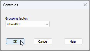
12. From the original resemblance matrix ('Resem1'), we can calculate distances among whole-plot centroids by clicking PERMANOVA+ > Distance Among Centroids..., and choosing the 'Grouping factor' as 'WholePlot', as shown below:

This will produce a new resemblance matrix of Bray-Curtis resemblances among the centroids for the 16 whole-plots, caled 'Resem2':

13. From the 'Resem2' matrix, produce a non-metric MDS plot by clicking Analyse > MDS > Non-metric MDS (nMDS).... Take all the defaults in the 'Non Metric MDS' dialog and click 'OK'. The resulting 2-dimensional nMDS plot (an item called 'Graph1' in the Explorer tree) is shown below.

As indicated by the pair-wise tests, we do see that most of the assemblages corresponding to unburned whole-plots (light blue diamond-shaped symbols) tend to occur towards the left-hand side of the ordination plot, whereas most of the assemblages corresponding to whole-plots burned at the highest frequency of every 2 years (the dark blue triangle-shaped symbols) tend to occur towards the right-hand side. However, this is not a super clear split, and there is rather high variation among whole plots within any of these treatments. The patterns on this ordination are quite consistent with the rather marginal pairwise test results that we obtained using PERMANOVA. In other words, from a practical point of view (omitting the two dominant grasses) there may only be somewhat minor differences in these plant assemblages caused by fire frequency, if any, at least for the time-scales examined in this study.

---

^¶Interaction terms are implied between any factors that are crossed with one another. By 'implied', we mean that they are conceivable, although they may not be estimable in all cases. That will depend on there being adequate replication. An interaction is not implied, however, between a given factor and another factor within which it is nested. For example, If we have Factor A and Factor B nested wtihin Factor A, then the only two terms in this model are A and B(A). Factor B clearly cannot interact with Factor A; therefore no A$\times$B interaction term is implied.

---

^†The closest we come to statistical significance at the 0.05 level is for the comparison of unburned plots (0 years) with plots burned most frequently, i.e., every 2 years. In that case, we have $t$ = 1.78 and the Monte Carlo p-value is 0.038, although the permutation p-value is 0.063, so this is a pretty marginal result.

---

^‡An alternative method to achieve the same result here would be to specify the 'Block' factor also as being of Type 'Subject/Whole-plot error'. This will automatically remove all interactions of the 'Block' factor with any other term(s) in the model.