10.4 Example: NZ fish assemblages

To further demonstrate the utility of main effects plots and interactions for multi-way study designs, we shall look at data from visual surveys of fish assemblages along the north-eastern coast of New Zealand completed annually (during the austral summer) over a period of 15 years, from 2001 - 2015, inclusive. In this study, divers did visual surveys at each of 4 locations ('BP' - Berghan Point, 'HP' - Home Point, 'Le' - Leigh, 'Ha' - Hahei), separated by hundreds of kilometres along the coast (Fig. 10.9). At each location, 4 sites (identified by GPS and revisited in each year) were sampled from each of two habitats: kelp forests ('k') and urchin-grazed barrens ('b') on near-shore rocky reefs. At each site, divers recorded the abundances of individual fish species observed in each of ten transects, with each transect measuring 25 m x 5 m. Over the 15-year period, a total of $p$ = 68 different fish species were recorded during the surveys. A subset of these data (from the initial 2 years of sampling) have been analysed and discussed previously by Anderson & Millar (2004) .

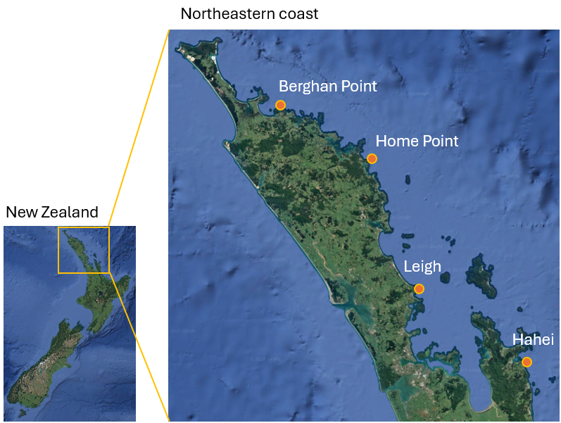
Fig. 10.9. Map of New Zealand and its north-eastern coast, showing the 4 locations where fish assemblages were surveyed annually from 2001-2015. Satellite images: Google Earth.

These data are located in the file 'NE_NZ_fish_counts.pri', found in the 'Example_P8' > 'NE_NZ_fish' folder. Note that data have been summed across the 10 transects to obtain a single measure of the multivariate fish assemblage at each site in every year.

Input data, apply pre-treatments, and calculate resemblances

1. Open up PRIMER and click File > Open... to bring in the data ('NE_NZ_fish_counts', found in the 'Example_P8' > 'NE_NZ_fish' folder).

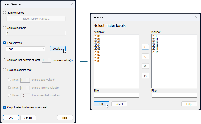
2. To simplify matters a little, we will analyse a subset of the data here. Select only years 2010 - 2015 inclusive. From the 'NE_NZ_fish_counts' sheet in PRIMER, click Select > Samples..., tick the box to '$\checkmark$ Output selection to new worksheet', then choose $\bullet$ Factor levels 'Year', and click the 'Levels' button (). In the 'Selection' dialog, click on each of the years from 2010 - 2015, then click on the right arrow () to move them over into the 'Include' box on the right, then click 'OK'. These steps are shown below:

The subsetted data will now be found in the sheet named 'Data1' in the Explorer tree. We shall use dispersion weighting (as many fish species naturally occur in aggregations/schools; see Clarke et al. (2006a) ), followed by a square-root transformation, to pre-treat the raw data prior to analysis. For the dispersion weighting, we need to provide several groups of replicates. A natural grouping factor to use here is the one we can create as a combination of the 3 main factors in this study design: Location, Habitat and Year. We first have to create this combined factor.

3. From the 'Data1' sheet, click Edit > Factors..., then click on the 'Combine' button (), followed by the 'Factors...' button (). In the 'Ordered Selection' dialog, click on each of the factors: 'Loc', 'Hab' and 'Year', in turn, then click on the right arrow () to move them over into the 'Include' box on the right, then click 'OK'(see below):

The resulting combined factor is called 'Loc-Hab-Year' and can be seen associated with the 'Data1' sheet when we click Edit > Factors... (it is in the last column).

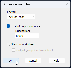
4. Now we can apply dispersion weighting on the basis of this combined factor. From the 'Data1' data sheet, click Pre-treatment > Dispersion Weighting... and in the resulting dialog, choose Factor: Loc-Hab-Year, then click 'OK'.

The dispersion-weighted data are provided in the sheet named 'Data2' in the Explorer tree.^¶

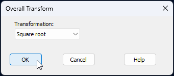
5. Next, apply a square-root transformation. From the 'Data2' sheet, click Pre-treatment > Transform(overall)... and choose Transformation: Square root, then click 'OK'.

The pre-treated data (square-root transformed dispersion-weighted values) are provided in the sheet named 'Data3' in the Explorer tree. We are ready now to calculate resemblances and proceed with analyses from there.

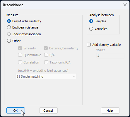
6. Calculate Bray-Curtis resemblances among all sampling units using the Bray-Curtis measure. From the 'Data3' sheet, click Analyse > Resemblance..., take all of the defaults, and click 'OK'.

The resulting resemblance matrix is in the item called 'Resem1' in the Explorer tree.

PERMANOVA

We shall begin by analysing these data using PERMANOVA on the basis of the Bray-Curtis resemblance matrix calculated from square-root transformed dispersion-weighted data ('Resem1'). Doing PERMANOVA first, in cases where there is a multi-factorial design, before we embark on ordinations, is often a good idea. The PERMANOVA partitioning will give us a quantitative comparative analysis of the relative importance of the factors (and their interactions) in our study design. Knowing which factors 'matter' (and which ones matter 'most') will help point us towards useful ordinations, to focus on the primary structuring factors of interest. Specifically, seeing the PERMANOVA output can help us decide which factors are worth looking at in more detail with main effects and interaction plots.

Create the PERMANOVA design file

There are four factors in this PERMANOVA design, as follows:

• Location (random with 4 levels: Berghan Point, Home Point, Leigh and Hahei)
• Habitat (fixed with 2 levels: kelp forest and urchin-grazed barrens)
• Year (random with 15 levels, a subset of 6 levels are examined here: 2010 - 2015 inclusive)
• Site (random and nested in Location and Habitat)

7. From the 'Resem1' matrix, click PERMANOVA+ > Create PERMANOVA Design.... In the resulting design file (called 'Design1'), click the 'Add row' button () three times, so there will be four rows in total here, then double-click inside each cell in the first column and choose the following factors in the study design ('Location', 'Habitat', 'Year', and 'Site'), in turn. Specify the 'Type' and 'Nested in' structure, as per the above 4-factor design by double-clicking inside the relevant cell in those columns for each factor in turn. The resulting design file, which mirrors the above articulated design, should look like this:

Run the PERMANOVA model

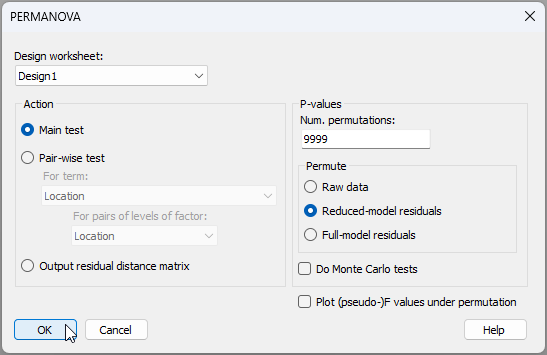
8. From the 'Resem1' matrix, click PERMANOVA+ > PERMANOVA..., make sure the 'Design worksheet:' is 'Design1', go with all of the default options for the rest, and click 'OK'.^‡

The resulting PERMANOVA output file ('PERMANOVA1') will look like this:

In a nutshell, we see here that all of the factors are statistically significant in this model. There is a significant three-way 'Location$\times$Habitat$\times$Year' interaction ($F_{15,119}$ = 1.32, $P$ < 0.01). This suggests that an interaction plot involving those three factors would be useful to examine.

Note that the 'Sq.root' column in the section labelled 'Estimates of components of variation' of the PERMANOVA output file gives us sizes of effects (in Bray-Curtis units) for each term in the model. For the main effects, this can be interpreted as a measure of the average (or 'standard') deviation of any given group centroid for that factor from the overall centroid.

Over and above the large variation among Sites (having a square-root estimated component of variation > 14 Bray-Curtis units), the main effects of Location and Habitat are also particularly strong (with square-root components of 16.5 and 15.7 Bray-Curtis units, respectively), while the main effects of Year were quite a lot smaller in size (7.5 Bray-Curtis units). This suggests that it would also be useful to examine a main effects plot involving those three factors (Location, Habitat and Year) for additional insights.

Ordinations

To help us visualise relationships among the sampling units, and potential structuring due to the spatial and temporal factors in the study design, we might consider plotting:

• an ordination of all sampling units from the full resemblance matrix;
• an ordination of centroids for the main factors: Location, Habitat and Year (a main effects plot);
• an ordination of centroids corresponding to combinations of factor levels for Location-by-Habitat-by-Year (an interaction plot).

Ordination of all sampling units

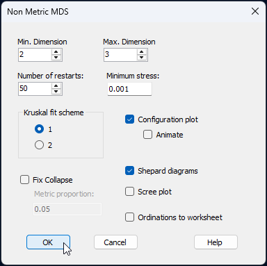
9. From the 'Resem1' matrix, click Analyse > MDS > Non-metric MDS (nMDS)..., take all of the default options and click 'OK'.

The resulting 2D nMDS ordination (provided in 'Graph1') looks like this (by default):

This is exceptionally messy and uninterpretable. Even if we remove the labels, no useful information can be taken from this ordination; for a start, the stress is just way too high (> 0.26). Even the best 3D nMDS solution has quite high stress (0.197) and looks like little more than a 'ball of fuzz'.

Main effects plot

10. To obtain a main effects plot, we first have to ammend our design file to remove the 'Site' factor, so as to focus our attention on the three main effects of interest here: 'Location', 'Habitat' and 'Year'. For this, simply click once on row 4 to highlight it, then click the 'Remove row' button () to remove the fourth (and final) row. The resulting 3-row design file (still called 'Design1') should look like this:^§

As an aside, note that the 'Type' of each factor has no particular relevance or impact on a main effects plot.

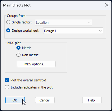
11. From the 'Resem1' matrix, click PERMANOVA+ > Centroid Plots > Main Effects Plot....

Choose (Groups from $\bullet$Design worksheet: Design1) and (MDS plot $\bullet$Metric). Also choose to $\checkmark$Plot the overall centroid, then click 'OK', like so:

The resulting main effects plot for these three factors is a threshold-metric MDS (called 'Graph5' in the Explorer tree), as shown below.

Outlined below are a number of observations we can draw from this ordination of main-effect centroids.

• First, the effects due to different locations are rather large, compared to the other factors. Fish assemblages from Leigh appear to be quite different from those at other locations, while fish assemblages from Berghan Point and Home Point (the two northern locations) are more similar to one another.
• Second, there is also quite a strong effect of Habitat. The effects of habitat on these fish assemblages (i.e., the distances from each of the habitat centroids to the overall centroid) appear to be similar in size to the location effects, on average, although they occur in a different direction in the multivariate space.
• Third, the inter-annual (temporal) effects are less important (smaller in size) than the spatial effects due to either the location or the habitat factors.
• Finally, and more generally, the lengths of the deviations of individual centroids for different levels of a given factor from the overall centroid, as may be estimated in this tmMDS ordination, are similar in size (and match the rank order of relative sizes) for these three main effects, as given in the PERMANOVA output file. That is, Location (~15-17 units) > Habitat (~13-15 units) > Year (~6-10 units). (Don't forget to add on the intercept value from the tmMDS to these in order to get the full picture regarding these distances). Of course, we mustn't forget that there is stress in this ordination diagram, so mean distances to the overall centroid won't match the effect sizes given by PERMANOVA precisely (we trust the quantitative information given by PERMANOVA more, where there is no stress involved), but for purposes of visualising the relative importance of these factors, this is really, nevertheless, a very helpful plot.

Interaction plot

12. To obtain a 3-way interaction plot, go to the 'Resem1' resemblance matrix in the Explorer tree, and click PERMANOVA+ > Centroid Plots > Interaction Plot....

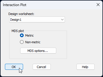
In the resulting dialog, choose (Design worksheet: 'Design1') and (MDS plot $\bullet$Metric), then click 'OK'.

This will produce a three-way interaction plot ('Graph9') that looks like this:

Note that what we see in this plot will depend on the order of the factors in the Design file. The default actions implemented by the Interaction plot routine are as follows:

• The first factor listed in the design file will be used to specify the colours of symbols.
• The second factor listed in the design file will be used to specify the shapes of symbols (i.e., varying across each colour).
• Thus, symbols are created as a combination of the first 2 listed factors in the design file.
• The third factor listed in the design file will be used to specify the labels.

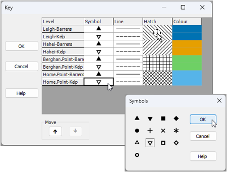
In this particular example, the 'Habitat' factor is a little difficult to discern via the default chosen symbol shapes (i.e., upward triangle vs downward triangle). As there are only 2 levels of the 'Habitat' factor, we could, instead, modify the default output by make the symbols corresponding to 'kelp' habitat open symbols instead of closed symbols (leaving the 'barren' habitat symbols as they are). This is easily done by clicking on the legend inside the graphic, and using the resulting dialog to modify the relevant symbols, like so:

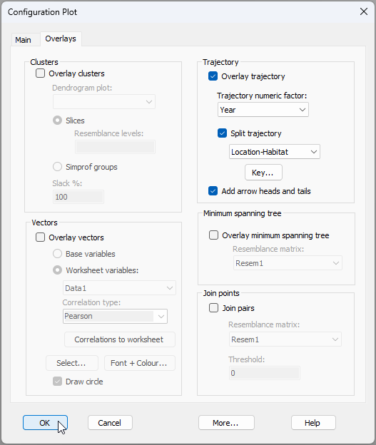
Another improvement to this graphic would be to superimpose a set of trajectories that link consecutive years for each Location-by-Habitat combination. Click Graph > Special.., and under the 'Overlays' tab, tick the box to $\checkmark$Overlay trajectory, with Trajectory numeric factor: Year and $\checkmark$Split trajectory by Location-Habitat, then click OK, as shown below:

The improved version of the interaction plot now looks like this:

This ordination is clearly far more useful than the nMDS ordination of all sampling units. The patterns we can see here include (but may not be limited to) the following:

• Fish assemblages at Leigh (dark blue) are quite distinct from those found at the other locations sampled along the coast, while the fish assemblages at the two northern locations (Berghan Point in light blue, and Home Point in green) are more similar to one another.
• There are clear differences in fish assemblages found in kelp forests vs those in barrens habitats (open symbols vs closed symbols, respectively), and these appear to be broadly similar effects across all 4 of the locations.
• Variation among years (e.g., look at the lengths of the trajectories) appears to differ for different locations and habitats. For example, temporal variation among years appears to be somewhat larger (years are more dispersed) in kelp habitats vs in urchin-grazed barrens habitats, and this difference is more marked for Leigh and Hahei, compared to Home Point and Berghan Point. Such patterns may easily explain the significant three-way interaction detected by PERMANOVA.

---

^¶A quick glance at the results file from this operation (called 'Dispersion weighting1' in the Explorer tree), shows how useful this pre-treatment operation was. A large number of these fish species have divisors that are a lot larger than 1, indicating they are highly aggregated. Many of these fish are indeed schooling fish, and some have numbers of individuals that are typically in the hundreds or even thousands within a single school. Recall that dispersion weighting downweights large abundance values for variables that have high variance-mean ratios, i.e., that are more erratic in their statistical behaviour. See Clarke et al. (2006a) for more details.

---

^†It is not strictly necessary to perform any kind of statistical analysis (whether it be PERMANOVA or ANOSIM, etc.) prior to creating ordination plots, of course. It is just sometimes helpful when there are a lot of factors. We can use the results from the PERMANOVA analysis to inform us of the most salient structuring factors in the study design and whether they interact, thus, pointing us towards what might be some of the most appropriate and useful ordinations to look at.

---

^‡ For this design, you will see a warning sign pop up, to highlight the fact the there is no replication at the lowest level. We know that there were, in fact, 10 replicate transects per site, but recall that we have summed these up to the site level for the analysis of fish communities.

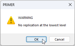
The pop-up warning means we cannot estimate the 'Year$\times$Site(Location$\times$Habitat)' interaction term because it is indistinguishable from the residual variation. You can click 'OK' in response to this warning, and PERMANOVA will continue with the analysis, automatically removing this inestimable high-order interaction from the design. It is worth bearing in mind that what is called 'Residual' in the resulting PERMANOVA output file is actually a mixture of the 'Residual' variation (from one site to another within a given year) and the potential variation due to the 'Year$\times$Site(Location$\times$Habitat)' interaction. This mixture is actually perfectly fine for generating all of the relevant tests we need for other terms of interest in our study design, so it is not something that will cause us to lose any sleep. All terms in our model are tested with perfect statistical rigour. As a further aside, note that 'Site' could optionally have been set up as a factor of type 'Subject/Whole-plot error', because we repeatedly went back to sample the same sites through time (every year), just as in a repeated-measures design (see section 8.3). If we had indeed chosen for 'Site' the 'Type' of 'Subject/Whole-plot error' in our design file, then no such warning would appear. However, we preferred here to include 'Site' as a nested factor, for transparency in the assumptions attending our model.

---

^§By the way, it is ok to keep all four factors in the design when you run the main effects plot, if you like. If you do that, there will be a centroid for every unique site in the resulting plot as well, so the ordination will just be a bit more busy to look at and make sense of. Keep in mind, if you do that, however, that the 'Site' centroids deviate around the 'Location-by-Habitat' centroids in the PERMANOVA model, and without the latter being plotted explicitly, site-level effects will be more difficult to read directly from the plot.