12.4 Bivariate normal example: NZ fish
To demonstrate the use of Hotelling's $T^2$ in a multivariate control-chart setting, it is useful to examine the method in 2 dimensions in Euclidean space (a bivariate system), which can be easily drawn and visualised. We shall examine bivariate patterns for two variables: richness and log-abundance, drawn from 15 years of annual underwater surveys of near-shore fish assemblages in northeastern New Zealand. This study was described earlier in section 10.4; see also Anderson & Millar (2004) .¶
Visualise bivariate patterns through time
The two variables we shall consider for this example are: the mean number of species (i.e., richness, 'S') and the mean of the total log abundance ('Log(N)'), calculated across the four sites sampled from urchin-grazed 'barrens' habitats only, and at the location of Home Point only.† It is quite reasonable to expect that these two variables will be approximately normally distributed, due to the central limit theorem. Let's start by considering a scatter plot of these two variables (Fig. 12.2). There is one sample point for each of the 15 years of sampling (so there are $n_c$ = 15 points in our baseline or reference set of samples). We can see that these two variables are positively correlated with one another; indeed, the Pearson correlation coefficient here is $r$ = 0.8128.
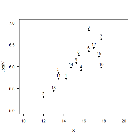
Fig. 12.2 Bivariate scatterplot of the average log total abundance per site ('Log(N)') and average richness per site ('S') for fish assemblages sampled in barrens habitats from Home Point, New Zealand. Numbers indicate 15 sequential years of sampling, from 2001-2015, inclusive.
Calculate the control-chart criterion
To this plot, we can add a trajectory of lines that connects the points corresponding to consecutive years through time. We can also calculate a multivariate control-chart criterion, Hotelling's $T^2$, at (say) the level of $\alpha$ = 0.05. This will circumscribe an ellipsoidal area in the 2D Euclidean space (Fig. 12.3). Any point falling inside the area would be considered 'in control', by reference to the 15-yr baseline set. In contrast, any point falling outside of that area would be considered 'out of control' - i.e., significantly different (at the level of $\alpha$ = 0.05) from the reference distribution.
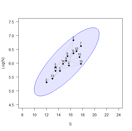
Fig. 12.3 Bivariate scatterplot as in Fig. 12.2, including a trajectory through time (grey lines) and an ellipsoidal region corresponding to the appropriate cut-off, $U_{CL}$ for a control-chart based on Hotelling's $T^2$ criterion (in blue).
Now let's suppose surveys are done in the 16th year, and we have a new value for each of S and Log(N) for that year. We can add this point to the plot. We will consider here two hypothetical outcomes: labeled as '16a' and '16b' in Fig. 12.4 and Table 12.1, below.
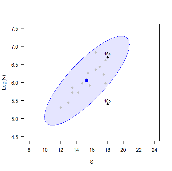
Fig. 12.4 Bivariate scatterplot as in Fig. 12.3, including the centroid from the first 15 years of sampling (in blue) and 2 hypothetical points that might be observed in year 16: labeled 16a (in control) and 16b (out of control).
Clearly, if 16a were the outcome, we would not consider this point to be 'unusual', given what we have observed over the prior 15 years. However, if 16b were the outcome, we would consider this to be very different indeed. Specifically, for 16b we can see that the log-abundance is much lower than what we would expect, given the level of richness observed. Now, the cut-off value for Hotelling's $T^2$ criterion in this bivariate example is $U_{CL}$ = 8.74 (at the level of $\alpha$ = 0.05). We have an observed value of $T^2 < U_{CL}$ for point 16a (in control), but, quite correctly, an observed value of $T^2 > U_{CL}$ for point 16b (out of control) (Table 12.1).
Table 12.1 Values of S, log(N), Euclidean distance to the baseline centroid, Hotelling's $T^2$ and the control chart outcome for two hypothetical points (16a and 16b), as shown in Fig. 12.4, that might occur in year 16.
| Sample | S | Log(N) | Euc. dist. to centroid | Hotelling's $T^2$ | Outcome |
|---|---|---|---|---|---|
| 16a | 18 | 6.700 | 2.712 | 2.51 | in control |
| 16b | 18 | 5.401 | 2.712 | 23.93 | out of control |
There are (at least) two important things to note about these two hypothetical outcomes.
- First, although they have the same Euclidean distance to the centroid of the baseline (reference) set of points, they have very different values for Hotelling's $T^2$ (Table 12.1). It is clear that taking a 'distance-to-centroid' approach completely ignores the shape of the data cloud, which is undesirable.‡ In other words, our approach here (using Hotelling's $T^2$) ensures that:
- the direction of the distance-to-centroid matters, not just its value; and
- the correlation structure is taken into account when we construct our criterion.
- Second, if we were to construct a univariate control chart for either of these individual variables alone, the values of 'S' and 'Log(N)' for 16b, when considered independently, are not particularly unusual at all, and the 16th year would not be identified as an outlier for either of these univariate variables. This example serves to show how it is not necessarily useful to think about multivariate data consisting of simply a 'stack' of individual univariate variables. How the variables covary with one another (hence affecting the shape of the data cloud) does matter.
Control chart for the bivariate example
We shall now show a control chart for a series of hypothetical data points for this example - projecting forward from the original 15 years of sampling for a further 10 years. We shall assert that the first 15 years provide a baseline set of samples. Hypothetical values for samples taken in 11 subsequent years (16 through 26) are to be compared with this baseline set, and are shown below (Fig. 12.5).
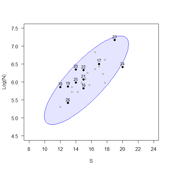
Fig. 12.5 Bivariate scatterplot of S and Log(N) for 15 baseline years (in grey), ellipsoidal region demarcating 'in-control' samples, based on Hotelling's $T^2$ criterion (in blue), and hypothetical samples for 11 subsequent years, 16 through 26 (in black).
The plot shows clearly that point 24 falls just outside the control-chart limit. Of course, if the system had more than just 2 dimensions, it would not be so easy to see outliers. A multivariate control chart of the data, including the upper control-chart limit, is the appropriate tool here (Fig. 12.6).
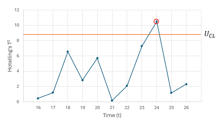
Fig. 12.6 Control chart showing the values of Hotelling's $T^2$ for each of 11 hypothetical samples obtained in years 16 through 26 (as shown in Fig. 12.5), by comparison with the 15-yr baseline set of samples, with the upper control-chart limit $U_{CL}$ (orange line). An out-of-control sample is detected in year 24 (red circle).
Although we have been looking here only at a bivariate example, a multivariate control chart of Hotelling $T^2$ values vs time will provide clear identification of 'out-of-control' samples, even for systems having a much larger number of dimensions. Note also that shrinkage can be used to estimate variance-covariance structure if the dimensionality of the system is large relative to sample size. However, thus far we have been operating only in Euclidean space, and we would clearly like now to extend these ideas to create control charts on the basis of a chosen dissimilarity measure, so as to accommodate species abundances (and other types of non-normal variables).
¶The data used for this example are in the file called 'NE_NZ_fish_counts.pri', found in the 'Example_P8' > 'NE_NZ_fish' folder.
†It is sensible for us to restrict our attention to a subset of the data like this, as the fish assemblages in different habitats and locations differed from one another.
‡The work by Anderson & Thompson (2004) introduced a control-chart criterion of distance-to-centroid in the space of a chosen dissimilarity measure. This works fine for situations where the cloud of 'in control' samples are approximately (hyper-)spherical in the multivariate space (isotropic), but it is really not ideal for situations where there are anisotropies (non-spherical shapes), as in the simple example shown here.