1-way layout (WA fish diet example)

Return to the W Australian fish diet data, introduced at the start of Section 4 and last seen under the Higher-d & scree plots heading of Section 8, showing MDS plots of dietary categories found in 65 (pooled) gut samples from 7 fish species. If the workspace WA fish ws is not available, re-open the data WA fish diets %vol.pri in C:\Examples v7\WA fish diets, exclude the samples A9, B3 and B4 (justifiable on the grounds of very low total gut content), standardise the samples, transform them with square root and take Bray-Curtis similarities, renaming this WA B-C sim. Re-run the nMDS and note that the number of replicates – the pools of fish from each species – is very uneven (from 3 to 15), as is the variability in diet for the different species (the dispersion of samples in the MDS space). Assumptions of balanced replication and the equivalent of ANOVA variance homogeneity are clearly not met here, but the ANOSIM test does not require such assumptions for its validity. Approximate balance in replication is still a good idea because it enhances the sensitivity of the tests, and comparable multivariate dispersion within each group makes interpretation simpler, but neither is possible here. ANOSIM tests the hypothesis that there are no dietary differences of any sort among the fish species. This null hypothesis can be rejected either because species require different food sources or because some have a much more variable diets than others, though they may feed on some of the same items – either or both reasons may contribute to rejection of the null.

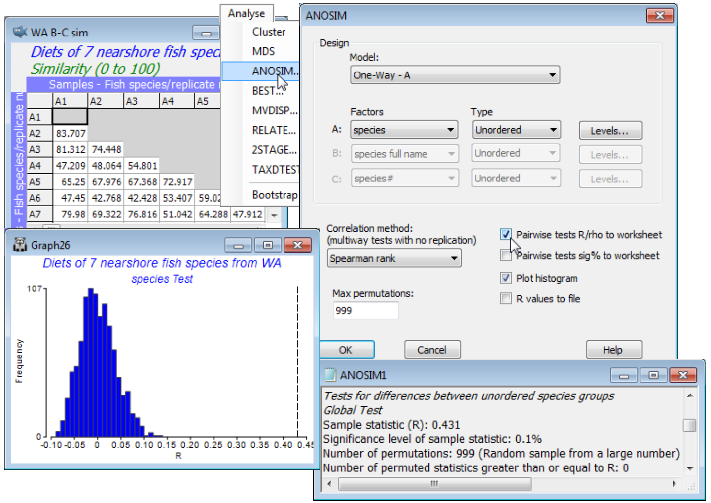
From the active window WA B-C sim, take Analyse>ANOSIM>(Model•One-Way - A)>(Factors A: species)>(Type Unordered), since clearly there is no prior expectation that if the diets differ then they can only do so along a steady gradient of change in a particular order of the fish species. (This is, however, exactly the expectation we have later when looking at the dietary changes of a single fish species at different stages of maturity, when the logical test will be an Ordered one). On the other choices, take (✓Pairwise tests R to worksheet) but leave the default settings for the remaining options, e.g. (Max permutations: 999) and Levels specifies that all 7 fish species are to be included. Three windows are created in the Explorer tree. ANOSIM1 is the results window, specifying the sheet and factor on which the test is performed, and giving the results of the overall ANOSIM test of the hypothesis of no differences in diet among any of the fish species, followed (when there are more than two groups, as here) by pairwise tests between the diets of every pair of fish species. The second output is a histogram of the permutation distribution of the ANOSIM test statistic, R, under the null hypothesis of the global test (though note that it is not the correct permutation distribution for any of the pairwise tests). The third output, requested here, is the set of observed pairwise R values held as a triangular (resemblance) matrix, and a similar option exists (not taken) to place the % significance levels for this set of pairwise tests in a further resemblance matrix.

This histogram is centred around zero – if there are no dietary differences then the average rank resemblance among and within groups will be much the same, and R (based on the difference between these two averages, see Chapter 6, CiMC) will be near zero. It can rise a little above (or below) zero by chance, when there are no differences among diets, but the histogram shows that it will never get larger than about R = 0.15. The true value of R for these data is also shown, as a dotted line, namely R = 0.43, and this is clearly much larger than any of the 999 permuted values, causing rejection of the null hypothesis at a significance level of at least 1 in 1000 (P<0.001, or as the PRIMER output prefers it: p<0.1%). The same information is repeated in the results window ANOSIM1 under the heading Global Test, namely the overall observed R statistic of 0.431, its significance level (p<0.1%), how many permutations were computed in order to determine this (999), and how many of those permutations gave an R value as large, or larger, than the observed R of 0.431 (none). The total number of possible permutations – distinct ways of dividing the 65 samples amongst the 7 fish species, keeping the same number of replicates for each species – is extremely large and is therefore not displayed. In other cases, with few replicates, this third row will give the exact number of possible permutations, and if this is less than the specified (Max permutations:           ) in the ANOSIM dialog box, then R will be evaluated for all possible permutations. Setting (Max permutations: 9999) will increase the significance level here to p<0.01% (it is clear from the histogram that, almost irrespective of how many permutations are chosen, a value as large as R = 0.43 will not be obtained by chance, so the significance level for the global test of no dietary differences can be made arbitrarily small, by increasing the number of permutations).