‘Ellipses’ for joint values of ($\Delta^{\scriptscriptstyle +}$, $\Lambda^{\scriptscriptstyle +}$))

The final option is to consider $\Delta^{\scriptscriptstyle +}$ and $\Lambda^{\scriptscriptstyle +}$ in combination, by plotting 95% probability contours for their joint distribution, under the null hypothesis of simple random (or frequency-based) selection from the master species list. Optionally, pairs ($\Delta^{\scriptscriptstyle +}$, $\Lambda^{\scriptscriptstyle +}$) from a real sample data matrix can be added. There may be some advantage in looking at both measures simultaneously because departures from expectation may reveal themselves as, say, lowish $\Delta^{\scriptscriptstyle +}$ and highish $\Lambda^{\scriptscriptstyle +}$ values, neither of which was significant on its own, but in combination outside the joint ($\Delta^{\scriptscriptstyle +}$, $\Lambda^{\scriptscriptstyle +}$) contours, for which $\Delta^{\scriptscriptstyle +}$ and $\Lambda^{\scriptscriptstyle +}$ might be negatively correlated. (The contours are drawn by approximating the simulations by a bivariate normal distribution in a transformed space, then back-transforming – Chapter 17, CiMC).

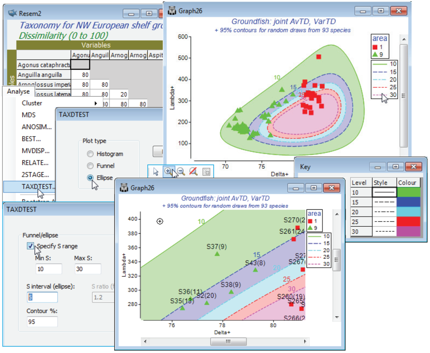
Just in order to create an example of how TAXDTEST can be run from a variable similarity matrix (such as might be found in a functional rather than taxonomic description of species relatedness, thus creating an Average Functional Distinctness diversity, AvFD, see Somerfield et al 2008, ICES J Mar Sci 65: 1462-1468), take Analyse>Similarity>(•Taxonomic), which simply returns a matrix of distances through the taxonomic tree. With this (Resem2) as the active window, run Analyse>TAXDTEST with option (Plot type•Ellipse) & (✓Use Sample data>Worksheet: Area 1 & 9) & (✓Specify S range)>(Min S: 10) & (Max S: 30) & (S interval (ellipse): 5), and selecting simple random sampling, i.e. uncheck (✓Use taxon frequency data). With (Contour %: 95), five contours will be produced, within which approximately 95% of the $\Delta^{\scriptscriptstyle +}$, $\Lambda^{\scriptscriptstyle +}$) pairs will lie, for s = 10, 15, 20, 25 and 30 random species draws. These contours must logically be concentric – if they do not look so it is certainly worth specifying more simulations, e.g. by (Max random selections: 9999) on the first TAXDTEST dialog screen. You may need to change the symbol types/colours again to get the first plot below, depending on which part of the Explorer tree you made the change to the Key area previously (if it was in the Area 1 & 9 sheet itself then this will be retained). There will now also be a key which controls the line type and line/shading colour for the 95% contours, and though this can be accessed from the Keys tab on the Graph Options dialog box, if changes are needed it is simplest just to click on the line key in the plot itself, taking you into the colour dialog.

For each sample, the idea is to visually interpolate between the contours for the two s values that straddle its observed number of species S, and determine whether that point is inside or outside its expected 95% contour (a Bonferroni-type correction could be used for the probability limits, or you should just bear in mind in interpreting the plot that 1 in 20 of points will fall outside 95% limits under random draws!). The conclusion here is again of a lower than expected average taxonomic distinctness (but mid-range VarTD) for area 9, and this is discrete from area 1, which has expected mid-range AvTD (and little evidence of VarTD being higher than expected). The interpretation of $\Delta^{\scriptscriptstyle +}$ and $\Lambda^{\scriptscriptstyle +}$ in general is covered in Clarke KR & Warwick RM 2001, Mar Ecol Prog Ser 216: 265-278 and Warwick RM & Clarke KR 2001, Oceanog Mar Biol Ann Rev 39: 207-231, and this study specifically in Rogers et al 1999, J Anim Ecol 68: 769-782 and Chapter 17 of CiMC.