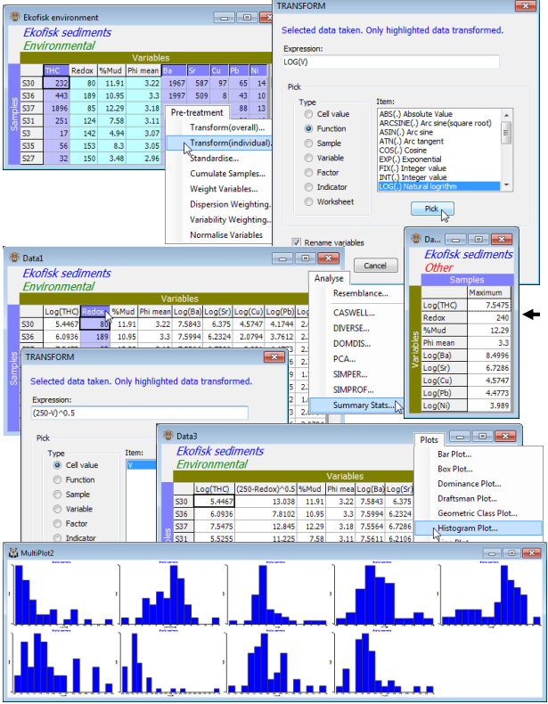
Transforming (individual)
Both the Draftsman and Histogram Plots show that several of the Ekofisk abiotic variables are highly right-skewed (tail to the right), and it would be wise, if we are to limit the distorting effects of outliers and normalise the data to a desired common measurement scale, to subject THC and the heavy metal concentrations to a strong transformation such as log(x). The particle size variables do not need further transformation ($\phi$ mean is already on a log scale). There is a case for regarding Redox as left skewed (it certainly has a large negative outlier), so we shall take the opportunity to demonstrate how to achieve a (mild) reverse power transform: $(a – x)^b$.
Highlight the THC, Ba, Sr, Cu, Pb, Ni variables and take Pre-treatment>Transform (individual). The transform operation itself can be any of the Transform(overall) options: square root, fourth root, log, reduction to pres/abs, using the Expressions: Sqr(V), V^0.25 ($\equiv$ Sqr(sqr(V)), log(1+V), PA(V) respectively, in which V (value) stands for any highlighted data entry (note that upper or lower case is not important in the expressions). But it is not limited to these: many other transforms can be constructed. In fact any expression using the Basic language syntax is permitted, involving operators: +, -, * (times), / (divide), ^ (power); functions: Sqr, Log (to base e) etc. as above, and Abs (absolute value), Atn (arctan), Exp (exponential), Int (integer part of a number) and many others; and even logical operators: =, <, >, <=, >=, which return –1 if true, 0 if false. (An example of the latter might be to draw attention to cells with large counts using an expression like V>1000). For a comprehensive list of expression options take Help on the Transform dialog box and click on Transform expression. Operations can extend still further, to generate new entries as combinations of samples or variables (and even factors or indicators or other worksheets), but examples of these are deferred until Section 11. In this case you simply need the Expression: log(V) which you can type directly into the Expression box or select the function from the Pick box: (Type•Function) & (Item: Log(.) Natural logarithm)>Pick. The action of the Pick button is to place the selected function around the default entry already in the Expression box (of just V). Check the expression is the one you intended and OK, to obtain a new sheet in which the concentration variables have been log transformed – their labels indicate this if you have left on the default of (✓Rename variables).
Note that the remaining variables have also been carried across to the new sheet but untransformed. This is the result of only highlighting the requisite variables rather than fully selecting them, with Select>Highlighted. (Had you done the latter then only the transformed variables would have been carried across to the new sheet, and you would have had to Select the others from the original sheet and Tools>Merge(d) them with the new, transformed variables). Now highlight the single Redox variable on the new sheet and Pre-treatment>Transform(individual)>(Expression: (250-V)^0.5). This reverses the distribution around a value just larger than its maximum, turning a mildly left-skewed shape into a mildly right-skewed one, and then the square root transformation will tend to remove that (mild) right-skewness – stronger would be to use log(250-V). Finding the maximum value for a variable is now easy with Analyse>Summary Stats>(For•Variables) & (✓Maximum). Again a new sheet is produced with the required mix of log, reverse square root and no transforms on different variables, and the efficacy of these in reducing the effects of outliers can be seen by another set of Plots>Draftsman Plot or Plots>Histogram Plot.

