Running the Bootstrap Averages routine

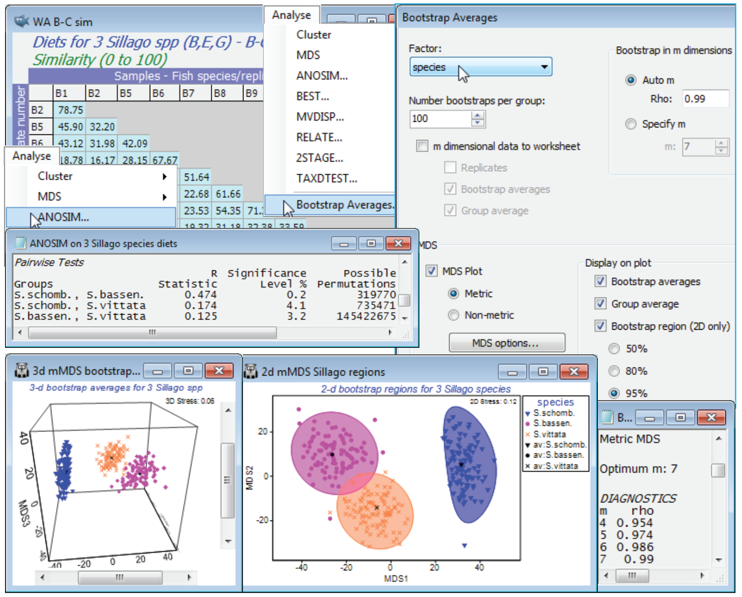
None of the above is necessary in order to create the means plot with regions based on bootstrap averages – it was included purely to note the initial steps the routine takes, under the automatic m option, in order to determine the mMDS dimensionality in which bootstrapping will take place. The Pearson $\rho$ values for increasing m = 4, 5, 6, … are sent to the results window, until they reach the given threshold (default $\rho \ge$0.99 or m gets to 10. These $\rho$ values will be displayed before starting the rest of the routine, namely the compute-intensive mMDS iterations for large numbers of points. So, run Analyse>Bootstrap Averages>(Factor: species) & (Number bootstraps per group: 100) & (•Auto m>Rho: 0.99) & (✓MDS plot•Metric) & (✓Bootstrap averages) & (✓Group average) & (✓Bootstrap region(2D only)•95%). There is also an option to send the m-dimensional data to a worksheet which is not the default and which you do not need to take here. This would allow the bootstrap averages and overall group averages to be placed together with the original replicate-level data (all in the reduced m dimensional space) for a further mMDS ordination. However, this will not usually be helpful – the original replicates will, in most cases, already fit poorly into low-d mMDS space, so compounding this by adding in several hundred points of bootstrap averages will only make matters worse, and an acceptable stress to allow the viewing of both replicates and a measure of uncertainty in the group means in a single ordination is rather unlikely. This should not be seen in too negative a light since, though the analogue of such a plot is perfectly feasible for univariate data, it is not seen very often there either!

As implied earlier, bootstrap averages are therefore calculated in m = 7 dimensional mMDS space, since the $\rho$ value has reached 0.99 at that point ($\rho$ is more or less guaranteed to increase as m gets larger, and could only not do so if a rather sub-optimal ordination has been generated for one of the trial values of m). The MDS section of the Bootstrap Averages dialog then determines what is done with the 300 averages (100 for each group) and the (Euclidean) distance matrix from their 7-d co-ordinate space. Clicking the MDS options button leads to the usual mMDS dialog and by default (as here) this will produce both a 2-d and 3-d mMDS ordination plot from these distances, the 2-d plot displaying the smoothed, nominal 95% regions described earlier (there is no option available for smoothed 3-d regions in the 3-d ordination). Note that the stress is much lower for both plots (0.12 for the 2-d and 0.06 for the 3-d) than for the original replicate-level space, even though there are 300 points rather than the original 38, primarily because these are plots of means of between 8 and 16 replicates and therefore have much lower sampling variability. The structure is also now (inevitably) much simpler, with three fairly well-defined groups of points.

There are several relevant points to note from these plots:
a) the smoothed regions, though they have to be convex, are not just ellipses – the back-transform from ellipses fitted in a transformed space gives good flexibility to mould the regions to the shape of the clusters of bootstrap averages;

b) the bias correction applied at this point tends to make the smoothed envelopes just slightly larger than the observed spread of 95 of the 100 bootstrap averages, though the effect is marginal, with the reasonably large n values (8 to 16) for the original replicates;

c) the spread of all three clusters of averages is relatively comparable but this is accidental and does not follow from any assumption of constant dispersion. The original replicate-level mMDS (though it needs to be interpreted cautiously with stress of 0.22) shows the blue triangles of S. schombergkii to have a somewhat less variable diet than the other two species, but it also has half the number of replicates (8, compared with 14 and 16) and therefore the variability will not decrease as much, as a result of the averaging – these two effects tend to cancel each other out;

d) the smoothed regions for S. bassensis and S. vittata marginally overlap, but in the 3-d solution, with its lower stress, the clusters seem disjunct (though abutting). However, you must resist the temptation to turn this into a hypothesis test. It is not even true in the simple univariate case (with full normality and constant variance assumptions), that if 95% confidence intervals overlap then their means are not significantly different – and here we have taken some trouble to point out the approximate nature (in several ways) of these nominal 95% envelopes. The formal tests here are those of ANOSIM – and PERMANOVA, since that works with the measurement scale of the dis-similarities (as mMDS does) rather than the rank values in ANOSIM. Here, as often, the tests give very similar results, with borderline significance for this pairwise difference (p<3% for both tests).