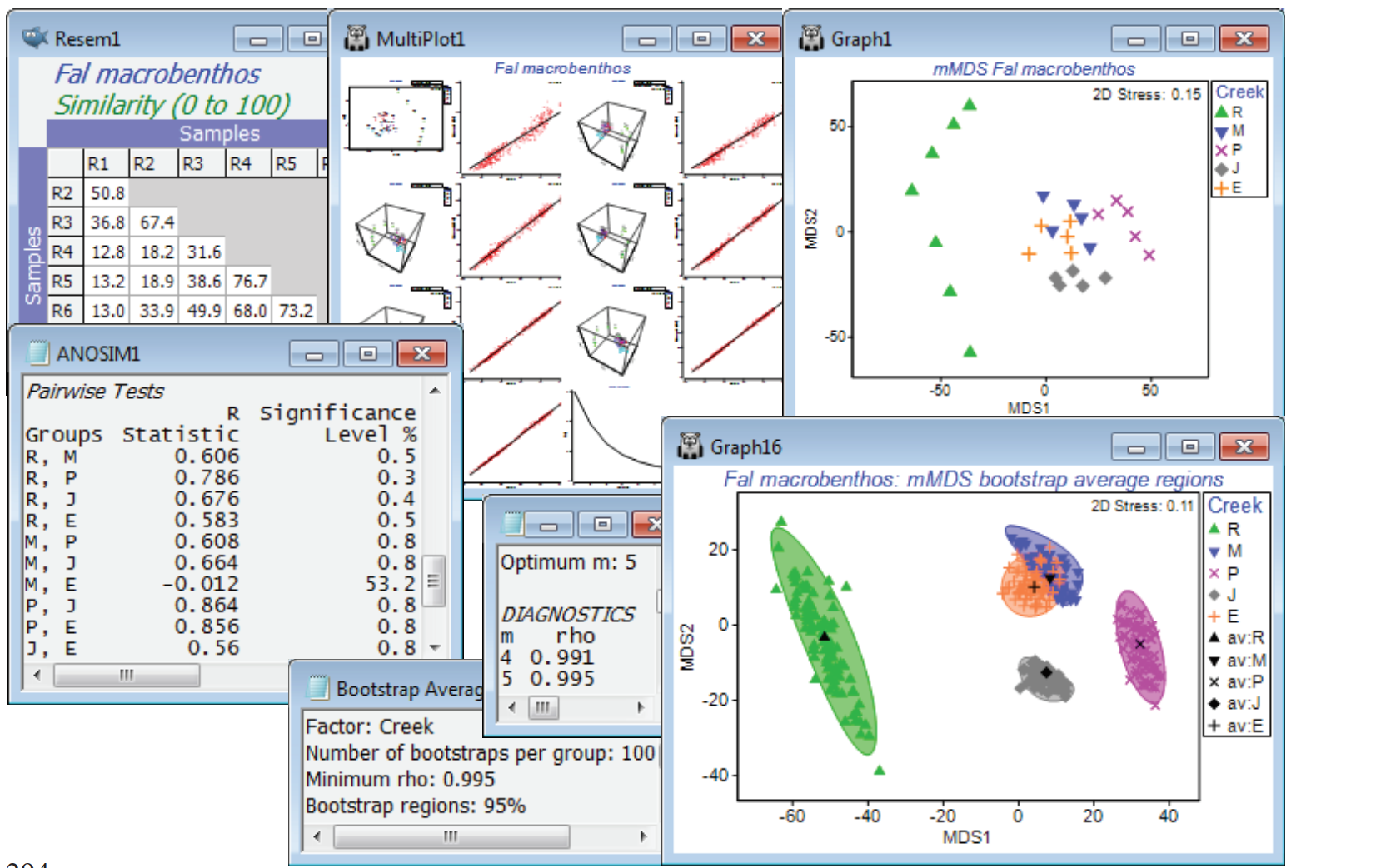
Bootstrap regions for Fal estuary macrofauna
A final example of bootstrap regions which do strongly overlap, and for which the hypothesis tests (such as ANOSIM) give no indication at all that the groups differ, is shown in Fig. 18.7 of CiMC. It can be reproduced here by opening the Fal macrofauna counts data file, in C:\Examples v7\Fal benthic fauna, into either a new workspace or Fal ws saved earlier (in which only the Fal copepod data was examined). The suite of data from these 27 locations from 5 creeks running into the Fal estuary, Cornwall, UK, were introduced in Section 4, and interest is in whether the differing levels of heavy metals in the sediments of these creeks, from historical tin and copper mining in their respective valleys, lead to differing macrofaunal (and meiofaunal) communities in those sediments. Fourth-root transform the Fal macrofauna counts, computing Bray-Curtis similarities and mMDS ordination of the replicate-level data. Running 1-way ANOSIM on the 5 creeks, with 7 replicates in Restronguet (R) and 5 for St Just (J), Pill (P), Mylor (M) and Percuil (E), gives strong differences, both in the global test (R = 0.49, p<0.1%) and in all pairwise tests (R>0.55, p<1%) except that between Mylor and Percuil (R = –0.01). Perusal of a means plot is therefore certainly justified.
The stress of 0.15 for the replicate level ordination is quite low for a metric MDS, and if the default range of dimensions requested is changed from 2-3 up to (for example) 2-8, it is clear from Shepard diagrams that by the time m=4 is reached, the m-dimensional mMDS distances are a very good fit to the full-dimensional resemblance matrix – in fact the later output of the bootstrap routine shows that this already gives a Pearson correlation of 0.991. Now enter the similarity matrix to Analyse>Bootstrap Averages>(Factor: Creek) and increase the number of bootstrap averages from the suggested default of 60 to nearer 100, depending on the speed of your machine. The (•Auto m) choice, with a $\rho$>0.99 threshold, as indicated, does lead to bootstrapping in m = 4 dimensions. You might wish instead to experiment with (•Specify m) at a higher, fixed level of 5 or 6, or increase the threshold in the automatic routine to $\rho$>0.995 or 0.999, but it will make negligible difference to the outcome in relation to the variation from run to run of the same m, resulting from the random differences in the bootstrap samples selected. (It is always a good exercise to repeat the bootstrap routine under the same conditions, and will discourage you from over-interpreting the minutiae of the region shapes!). Though the below did use 100 bootstraps from each creek, a replication level of only n=5 in four of the creeks must be considered absolutely minimal, and the striations in the bootstrap average points, which are just discernible in the plot, result from the fact that there are then only a possible 126 bootstrap averages (not equally likely) and several will have been created more than once. (The n=7 for Restronguet gives 1716 possibilities and thus more of a continuum of average values). So the plots should again be interpreted with caution, but the pattern of differences among creeks is clear, and fully consistent with the hypothesis testing.

