1.12 Monte Carlo P-values (Victorian avifauna)
In some situations, there are not enough possible permutations to get a reasonable test. Consider the case of two groups, with two observations per group. There are a total of 4 observations, so the total number of possible re-orderings (permutations) of the 4 samples is 4! = 24. However, with a groups and n replicates per group, the number of distinct possible outcomes for the F statistic in the one-way test is $(an)! / [ a! ( n ! ) ^ a ]$ (e.g., Clarke (1993) ), which in this case is: $(4)! / [2! (2!)^2] = 3 $ unique outcomes. This means that even if the observed value of pseudo-F is quite large, the smallest possible P-value that can be obtained is P = 0.333. This is clearly insufficient to make statistical inferences at a significance level of 0.05.
An alternative is to use the result given in Anderson & Robinson (2003) regarding the asymptotic permutation of the numerator (or denominator) of the test statistic under permutation (see equations (1) and (4) on p. 305 of Anderson & Robinson (2003) ). It is demonstrated (under certain mild assumptions17 that each of the sums of squares has, under permutation, an asymptotic distribution that is a linear form in chi-square variables, where the coefficients are actually the eigenvalues from a PCO of the resemblance matrix (see chapter 3). Thus, chi-square variables can be drawn randomly and independently, using Monte Carlo sampling, and these can be combined with the eigenvalues to construct the asymptotic permutation distribution for each of the numerator and denominator and, thus, for the entire pseudo-F statistic, in the event that too few actual unique permutations exist.
A case in point where such an issue arises is given by a study of Victorian avifauna by Mac Nally & Timewell (2005) . The data consist of counts of p = 27 nectarivorous bird species at each of eight sites of contrasting flowering intensity within the Rushworth State Forest in Victoria, Australia. One pair of sites had heavy flowering (‘good’ sites), another pair had intermediate flowering (‘medium’ sites), and a third pair had relatively little flowering (‘poor’ sites). Two sites near the good sites (‘adjacent’ sites), were also selected to explore possible “spill-over” effects. Sites were sampled using a strip transect method and data from four surveys were summed for each site ( Mac Nally & Timewell (2005) ). The data are located in the file vic.pri in the ‘VictAvi’ folder of the ‘Examples add-on’ directory. An MDS ordination of the 8 sites on the basis of the binomial deviance dissimilarity measure ( Anderson & Millar (2004) ) indicates potential differences among the four groups of sites in terms of their avifaunal community structure and an overall gradient from good to poor sites (Fig. 1.12).
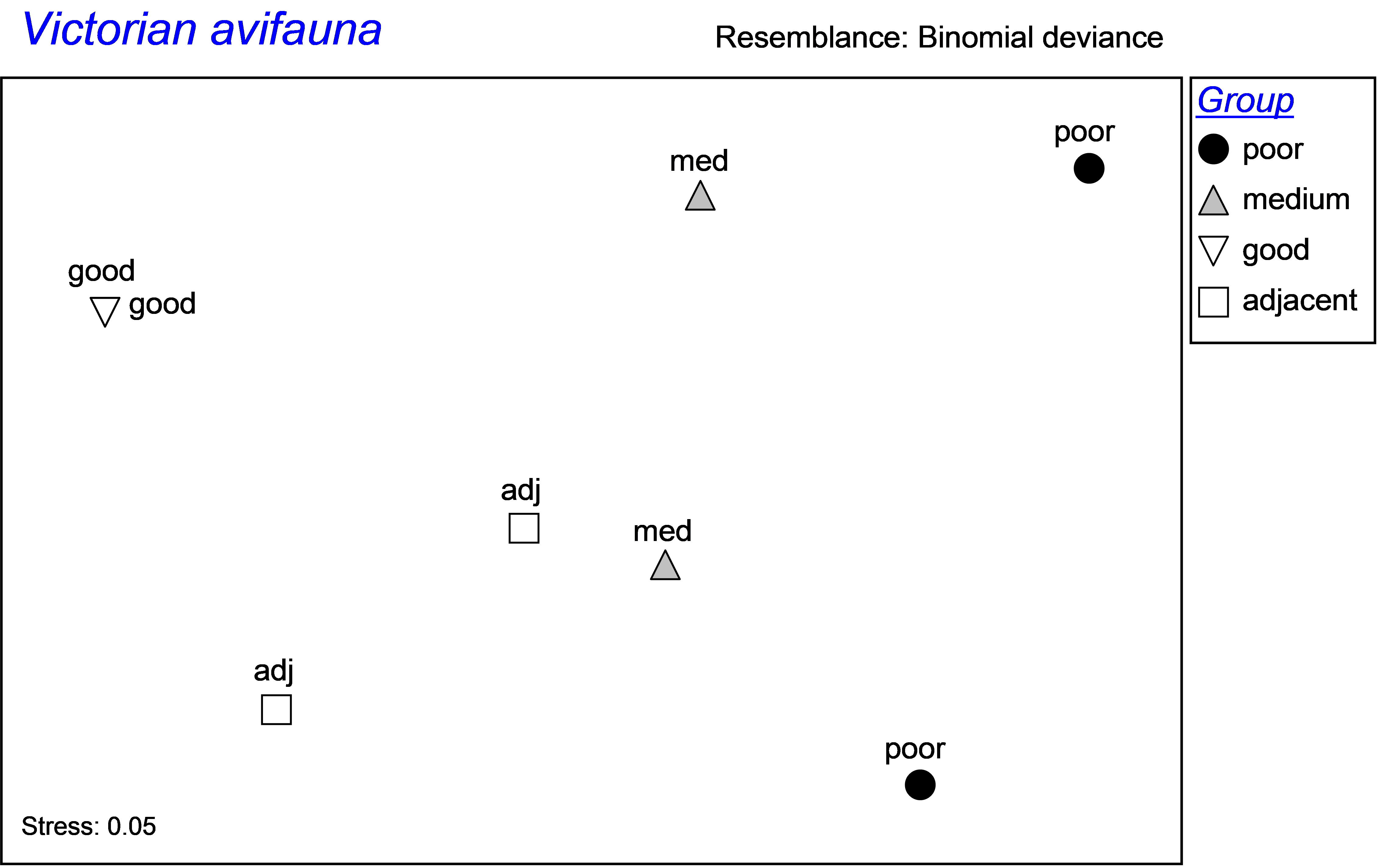 Fig. 1.12. MDS plot of Victorian avifauna at sites with different flowering intensities.
We have a = 4 and n = 2, so there will be a total of $(8)!/[4!(2!)^4] = 105$ unique values of the pseudo-F ratio under permutation for the main PERMANOVA test. This will provide some basis for making inferences from the P-value. For the pair-wise tests, however, there will be only 3 unique values under permutation, so obtaining Monte Carlo P-values would clearly be useful for these. To obtain Monte Carlo results, in addition to the permutation P-values, simply choose ($\checkmark$Do Monte Carlo tests) in the PERMANOVA dialog.
For the Victorian avifauna, the PERMANOVA main test suggests that there are significant differences in bird communities among the four types of sites (Fig. 1.13). The permutation and Monte Carlo P-values are quite similar in value (‘P(perm)’ = 0.02 and ‘P(MC)’ = 0.03) and note how the routine also faithfully shows that 105 unique values of pseudo-F were obtained under permutation (‘Unique perms’).
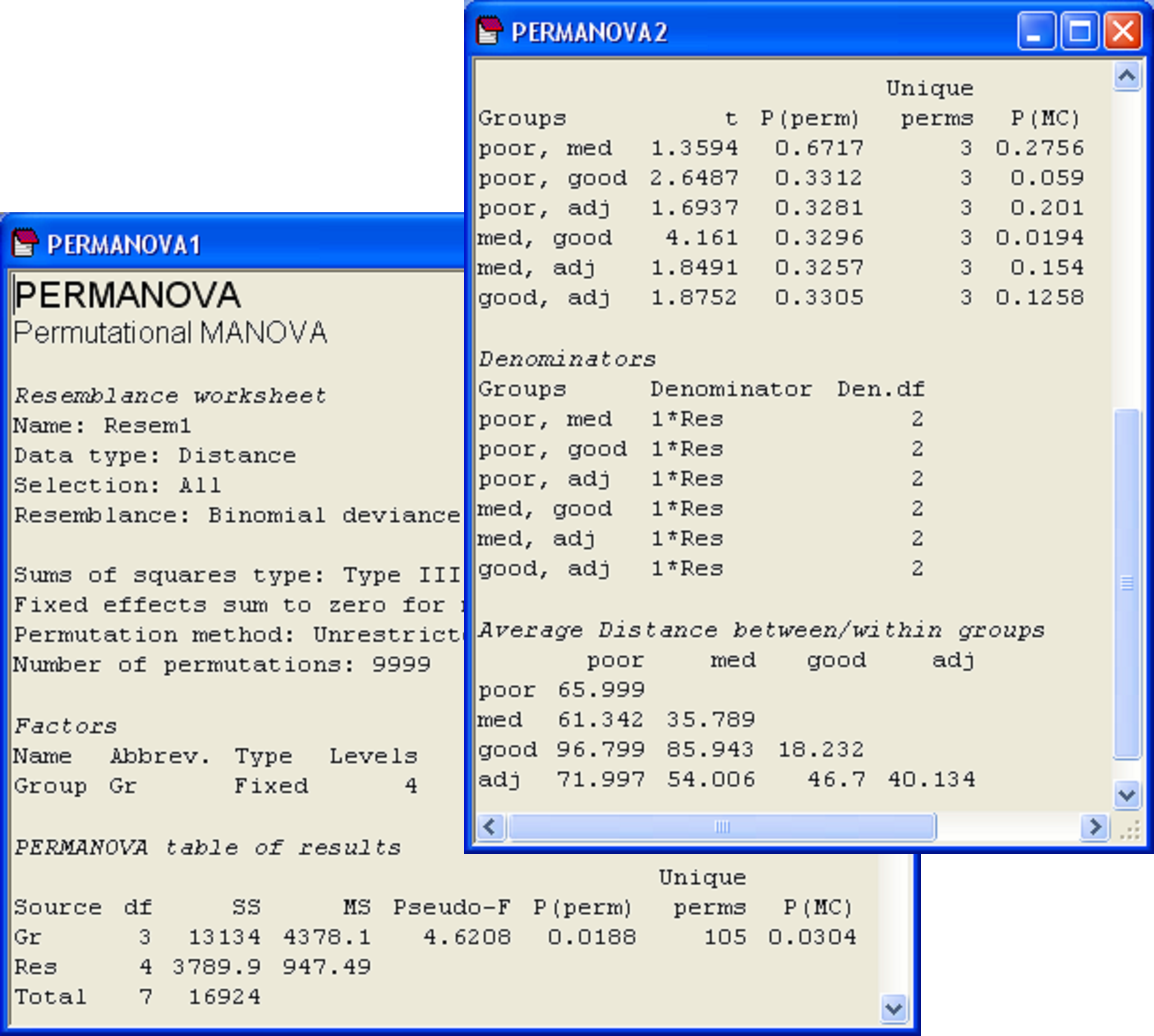 Fig. 1.13. PERMANOVA results for the main test and pair-wise tests for the Victorian avifauna, including Monte Carlo P-values.
The P-values for the pair-wise tests are virtually meaningless in this example, as there are only 3 unique possible values under permutation in each case. However, the Monte Carlo P-values are clearly much more valuable here and can be interpreted. Sites with medium flowering intensity appear to differ significantly from those with good flowering intensity (‘P(MC)’ = 0.02), which is also reflected in the relative size of the pseudo-t statistic (= 4.16). None of the other P-values were less than 0.05, although the comparison of poor with good sites came close (‘P(MC)’ = 0.06). One possible reason this latter comparison did not achieve a higher t statistic is because of the large within-group variation of the poor sites (average within-group distance = 66.0, Fig. 1.13).
If the number of unique permutations is large (say, 100 or more), then the permutation P-value should be preferred over the Monte Carlo P-value, as a general rule, because it will provide a more accurate test. The Monte Carlo P-values are based on asymptotic theory (albeit a very robust theory that generates distributions for test statistics which are specific to each dataset), so they rely on large-sample approximations. When there are a large number of possible permutations, then the Monte Carlo and permutation P-values should be very similar, essentially converging on the same answer. When, on the other hand, there are very few possible permutations, then the two P-values may be quite different (as seen in the Victorian avifauna example), in which case the Monte Carlo P-value should probably be used in preference. Although the Monte Carlo P-value is, at least, interpretable in cases such as these, it is only an approximation which relies on the central limit theorem, so clearly we shouldn’t get too carried away with our statistical inferences and interpretation of P-values from studies having such small sample sizes18.
In multi-factor designs (discussed below), it is not always easy to calculate how many unique permutations there are for a given term in the model. It depends not only on the permutation method chosen, but also potentially depends on other factors in the model, how many levels they have and whether they may, under permutation, coincide with the term being tested in serendipitous ways. Therefore, for each test, PERMANOVA simply keeps track of how many unique values of the test statistic it encounters out of the total number of random permutations done. Armed with this information (‘Unique perms’), it is then possible to judge how useful the permutation P-value given actually is, under the circumstances.
17 The essential assumptions here are (a) that the observations of multivariate observations under permutation are independent and identically distributed, (b) that the distances are not just governed by a couple of very large ones (so that the central limit theorem can apply) and (c) that the distances are not too discontinuous – so a small change in the data would not produce a large change in the distance (sensible distance functions satisfy this). See Anderson & Robinson (2003) for details.
18 Unfortunately, it is precisely in these situations where sample sizes are small and we would like to use the Monte Carlo P-value that the asymptotic approximations assumed by this approach are actually the most precarious! A clear topic for further study is to discover under what conditions, more specifically, the Monte Carlo P-values may become unreliable.