2.11 Dispersion in nested designs (Okura macrofauna)

In many situations, the experimental design is not as simple as a one-way analysis among groups. For more complex designs, several tests of dispersion may be possible and relevant at a number of different levels. The sort of tests that will be logical to do in any given situation will depend on the design and the nature of existing location effects (if any) that were detected by PERMANOVA. This is particularly the case when factors can interact with one another (see the section on crossed designs below). First, however, we shall consider relevant tests of dispersion that might be of interest in the case of a nested experimental design. For simplicity, we shall limit our discussion here to the two-factor nested design, although the essential principles discussed will of course apply to situations where there are greater numbers of factors in a nested hierarchy.

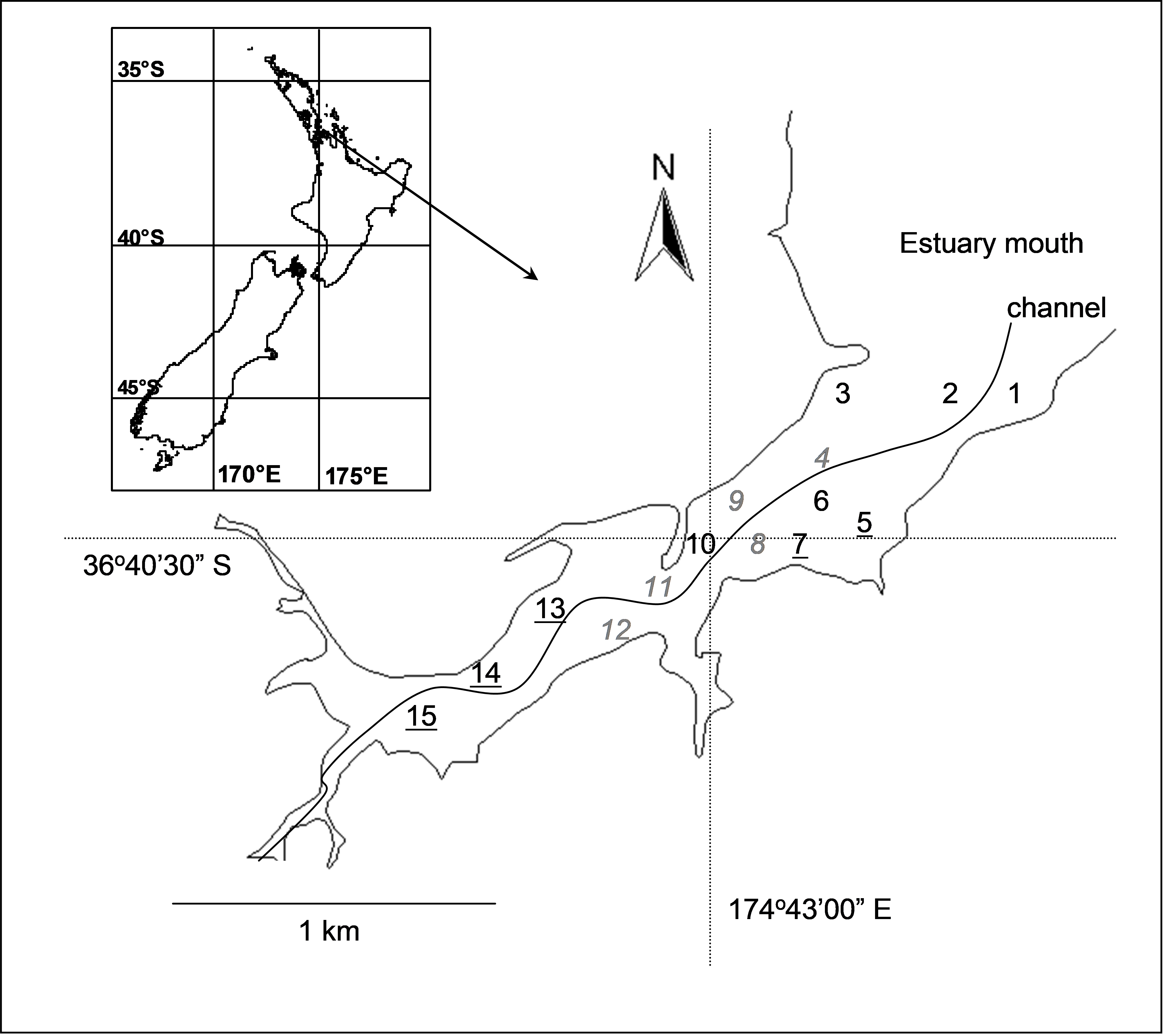Fig. 2.10. Okura estuary, with the 15 sites for sampling of benthic fauna labeled: high depositional sites are underlined, medium depositional sites are in italics and low depositional sites are in normal font.

Consider the experimental design described by Anderson, Ford, Feary et al. (2004) investigating the potential effects of different depositional environments on benthic intertidal fauna of the Okura estuary in New Zealand. The hydrology and sediment dynamics of the estuary had been previously modeled ( Cooper, Green, Norkko et al. (1999) , Green & Oldman (1999) ), and areas corresponding to high, medium or low probability of sediment deposition were identified. There were n = 6 sediment cores (13 cm in diameter × 15 cm deep) obtained from random positions within each of 15 sites along the estuary, with 5 sites from each of the high, medium and low depositional types of environments (Fig. 2.10). Sampling was repeated 6 times (twice in each of three seasons in 2001-2002), but we shall focus for simplicity on the following spatially nested design for the first time of sampling only:

• Factor A: Deposition (fixed with a = 3 levels, high (H), medium (M) or low (L)).

• Factor B: Site (random with b = 5 levels, nested in Deposition).

The design was balanced, with n = 6 replicate cores per site for a total of N = a × b × n = 90 samples obtained at each time. The data (counts of p = 73 taxa) are located in the file okura.pri in the ‘Okura’ folder of the ‘Examples add-on’ directory. We shall follow Anderson, Ford, Feary et al. (2004) and perform the analysis on the basis of the Bray-Curtis measure on log(x+1)-transformed abundances. An MDS plot of the data from time 1 only (Fig. 2.11) revealed a fairly clear pattern to suggest that assemblages from different depositional environments were distinguishable from one another, especially those from sites having relatively high probabilities of deposition.

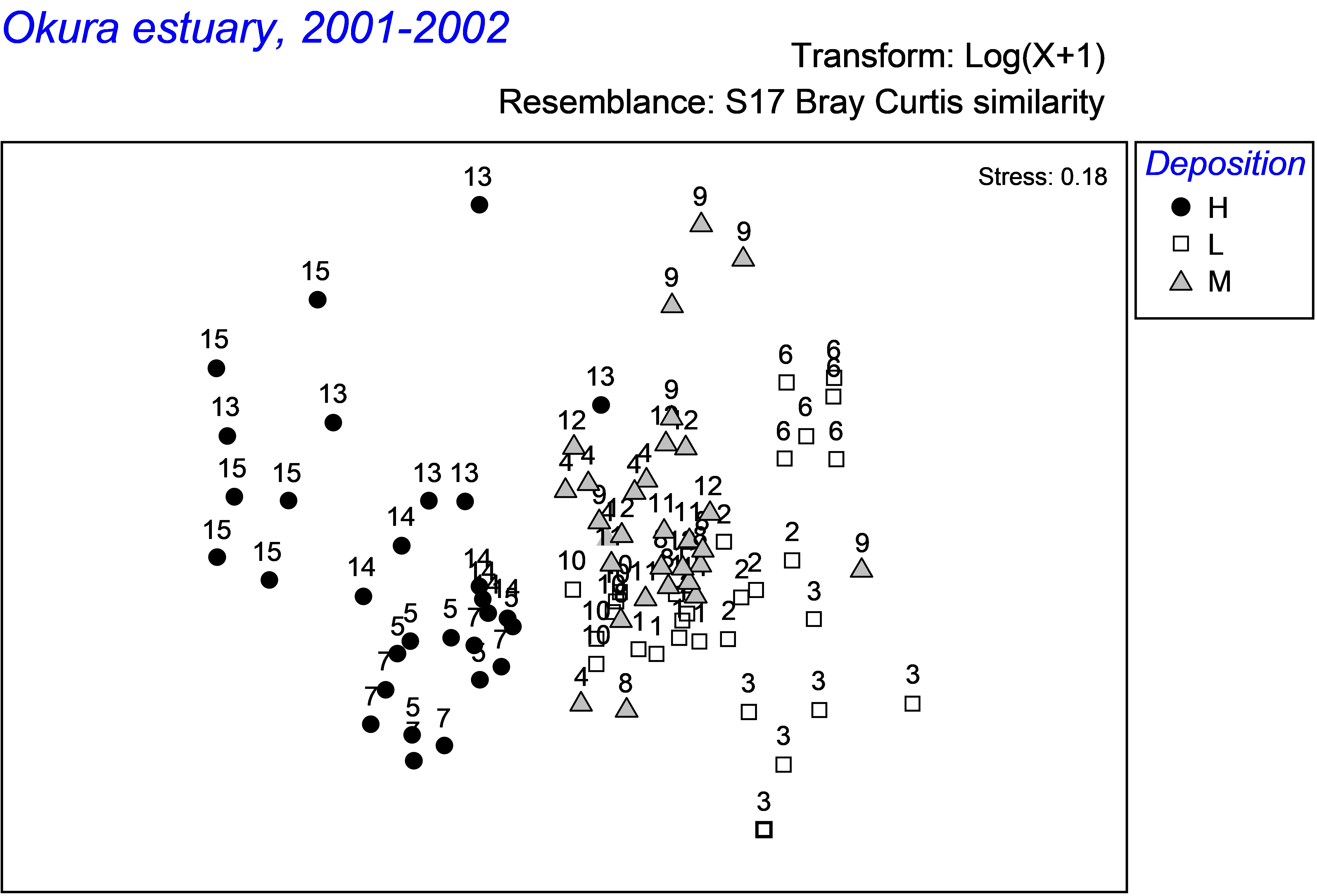Fig. 2.11. MDS of assemblages of intertidal soft-sediment infauna from Okura estuary at each of 15 sites (numbered as in Fig. 2.10) having high (H), medium (M) or low (L) probabilities of sediment deposition.

For a design such as this, there are two levels at which we may wish to think about relative dispersions. First, are the multivariate dispersions among the 6 cores within a site different among sites? Second, are the multivariate dispersions among the 5 site centroids different among the three different depositional environments? Another (third) possibility might be to compare the dispersions of the 5 × 6 = 30 cores across the three depositional environments. However, such a test would only really be logical if there were no differences in location among sites (i.e. no significant ‘Site’ effects in the PERMANOVA).

First, consider the variability among cores within each site. For these particular data, the 15 sites are labeled 1-15 according to their position in the estuary (Fig. 2.10). Thus, to compare dispersions of assemblages in cores across sites, we simply run PERMDISP on the factor ‘Site’ for the full resemblance matrix. Note that these a × b = 15 cells correspond to the lowest-level cells in the design. If the sites had been labeled 1-5, that is, if the sites had been given the same labels within each of the depositional environments (even though they are different actual sites, being nested), then we would have to first create a new factor corresponding to the fifteen cells (all combinations of factors A and B) by choosing Edit > Factors > Combine.

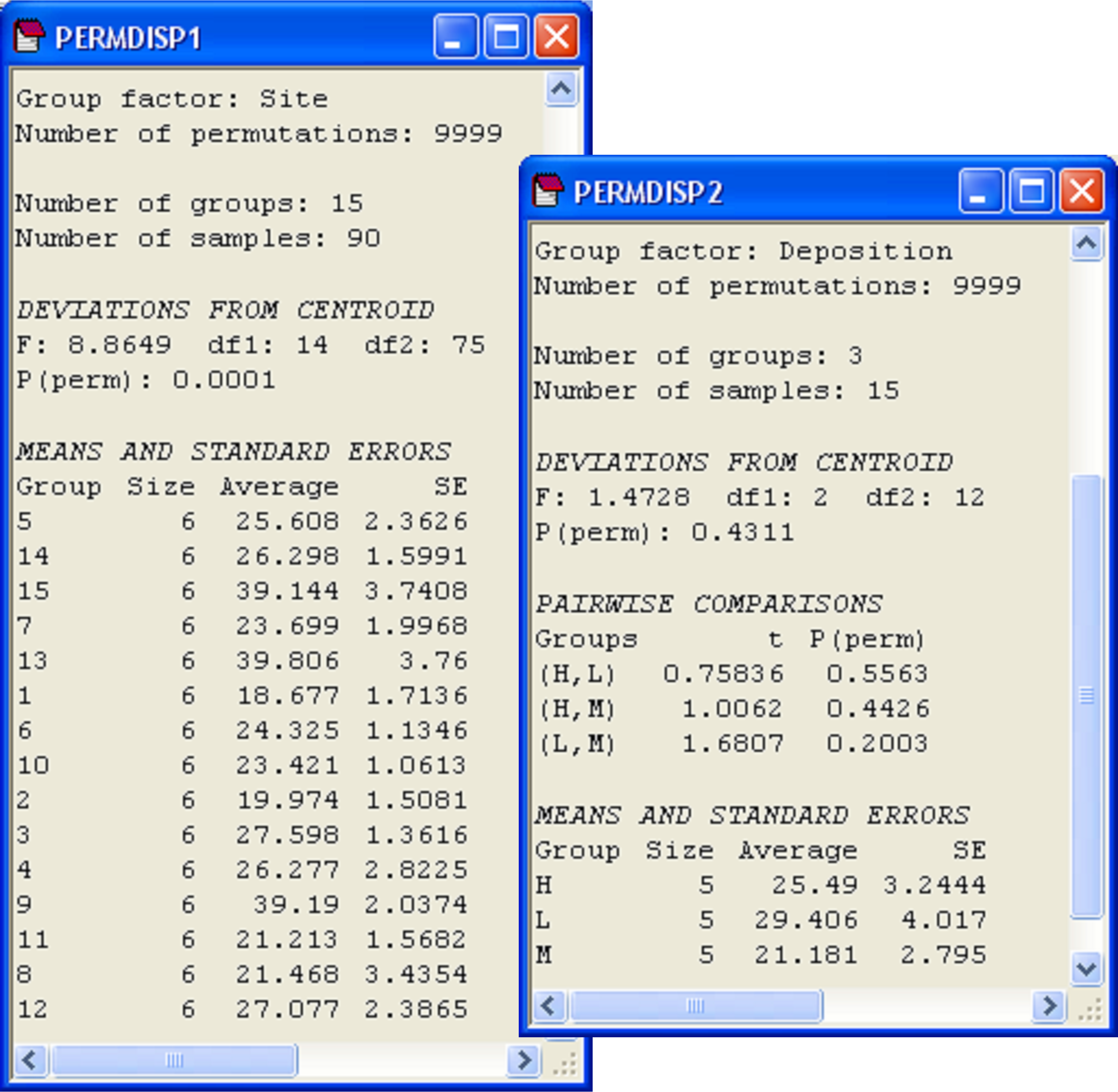Fig. 2.12. PERMDISP analyses for a nested design done at two levels: comparing variability among cores across sites (left) and comparing variability among sites across depositional environments (right).

This first PERMDISP analysis reveals that the dispersion among cores varies significantly from site to site (Fig. 2.12, F = 8.86, P < 0.001). As ‘Site’ is a random factor, we are not especially interested in performing pairwise comparisons here, so these have not been done. There is heterogeneity in dispersions among cells and examining the output reveals that the average distance-to-centroid in Bray-Curtis space within a site generally varies from about 18 to 27%. Three of the sites, however, have an average distance-to-centroid of nearly 40% (Fig. 2.12).

Next, we shall consider the second question posed above: are there differences in the dispersions of the 5 site centroids for different depositional environments? Before proceeding, we first need to obtain a distance matrix among the site centroids. Recall, however, that the centroids in Bray-Curtis (or some other non-Euclidean space) are not the same as the arithmetic centroids calculated on the original variables. Thus, unfortunately, we cannot calculate the site centroids by going back to the raw data and just calculating site averages for the original variables. Instead, we shall use a new tool available as part of the PERMANOVA+ add-on, which calculates a resemblance matrix among centroids for groups identified by a factor in the space of the chosen resemblance measure. To do this for the present example, click on the resemblance matrix and then choose PERMANOVA+ > Distances among centroids… > Grouping factor: Site, then click ‘OK’. The resulting resemblance matrix contains the correct Bray-Curtis dissimilarities among the site centroids, which have been calculated using PCO axes (see the section Generalisation to dissimilarities above). Just to re-iterate, these centroids are not calculated on the original data, they are calculated on PCO axes obtained from the resemblance matrix, in order to preserve the resemblance measure chosen as the basis of the analysis.

To visualise the relative positions of centroids in multivariate space, choose Analyse > MDS from this resemblance matrix among centroids. Conveniently, PRIMER has retained all of the factors and labels associated with these points, so we can easily place appropriate labels and symbols onto the centroids in the plot. The dispersions of the site centroids appear to be roughly similar for the three depositional environments (H, M and L, Fig. 2.13), and indeed the test for homogeneity of dispersions revealed no significant differences among these three groups (Fig. 2.12, F = 1.47, P = 0.43). Note that ‘Deposition’ is a fixed factor and so we would indeed have been interested in the pair-wise comparisons among the three groups (had there been a significant F-ratio). This is why the option $\checkmark$Do pairwise tests was chosen; these results are also shown in the output (Fig. 2.12).

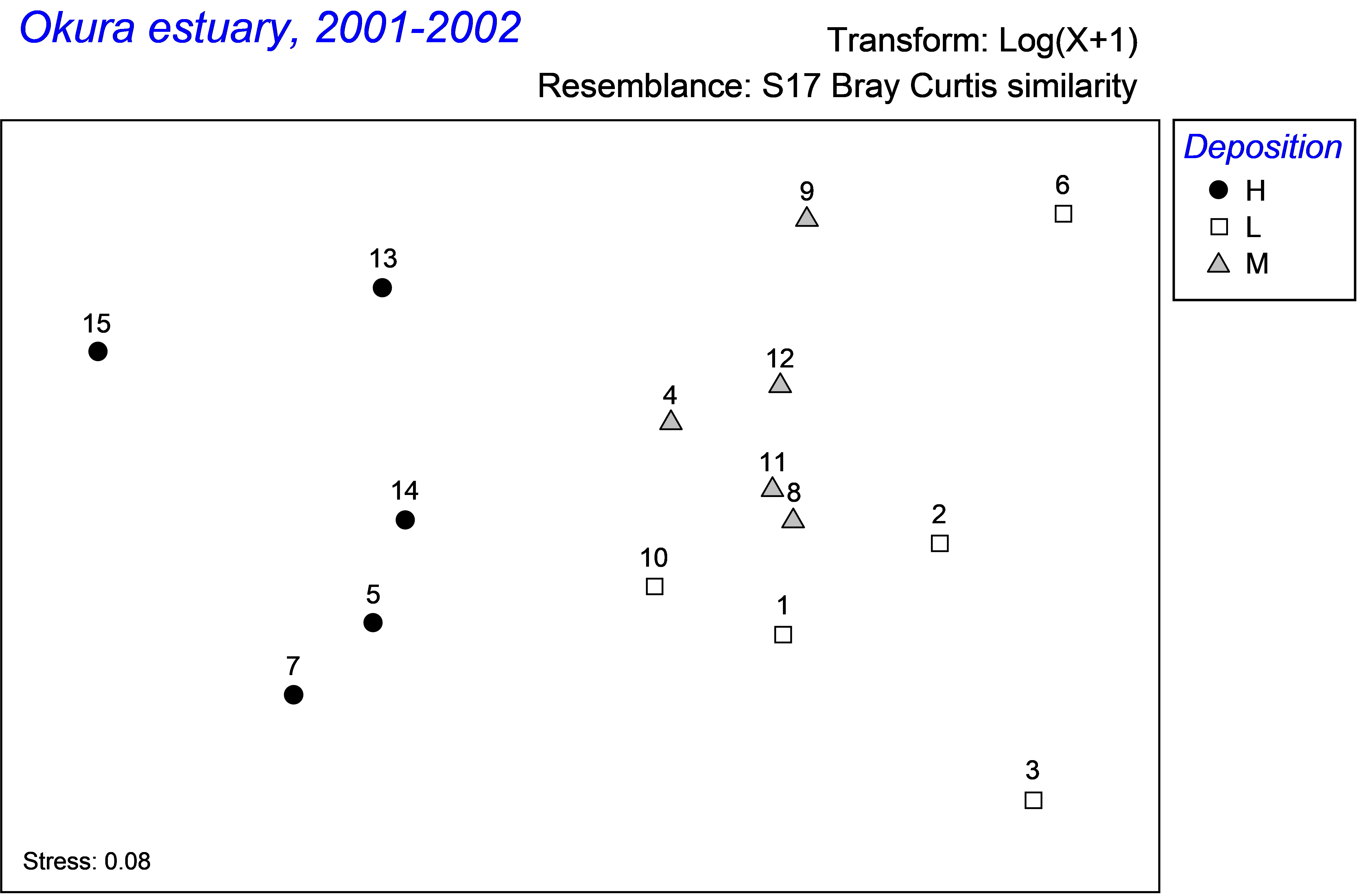Fig. 2.13. MDS of site centroids for the Okura data obtained from PCO axes on the basis of the Bray-Curtis resemblance measure of log(x+1)-transformed abundances.

Finally, we may consider the third question above: are there differences in dispersions among cores (ignoring sites) for the three depositional environments? Such a question only makes sense if sites have no effects. However, the results of the two-factor PERMANOVA for this experimental design reveals that ‘Site’ effects are highly statistically significant (pseudo-F = 5.49, P < 0.001, Fig. 2.14). Therefore, there is no logical reason to consider the multivariate dispersion of cores in a manner that ignores sites. As an added note of interest, the PERMANOVA test of the factor ‘Deposition’ in the two-factor nested design yields the same results as a one-way PERMANOVA for ‘Deposition’ using the resemblance matrix among site centroids (pseudo-F = 4.56 with 2 and 12 df, P < 0.001, Fig. 2.14). This clarifies how the nested model effectively treats the levels of the nested term (in this case, ‘sites’) as replicates for the analysis of the upper-level factor. Note that this equivalence would not hold if the centroids had been calculated as averages from the raw (or even the transformed) original data, which further emphasises that the centroids obtained using PCOs are indeed the correct ones for the analysis.

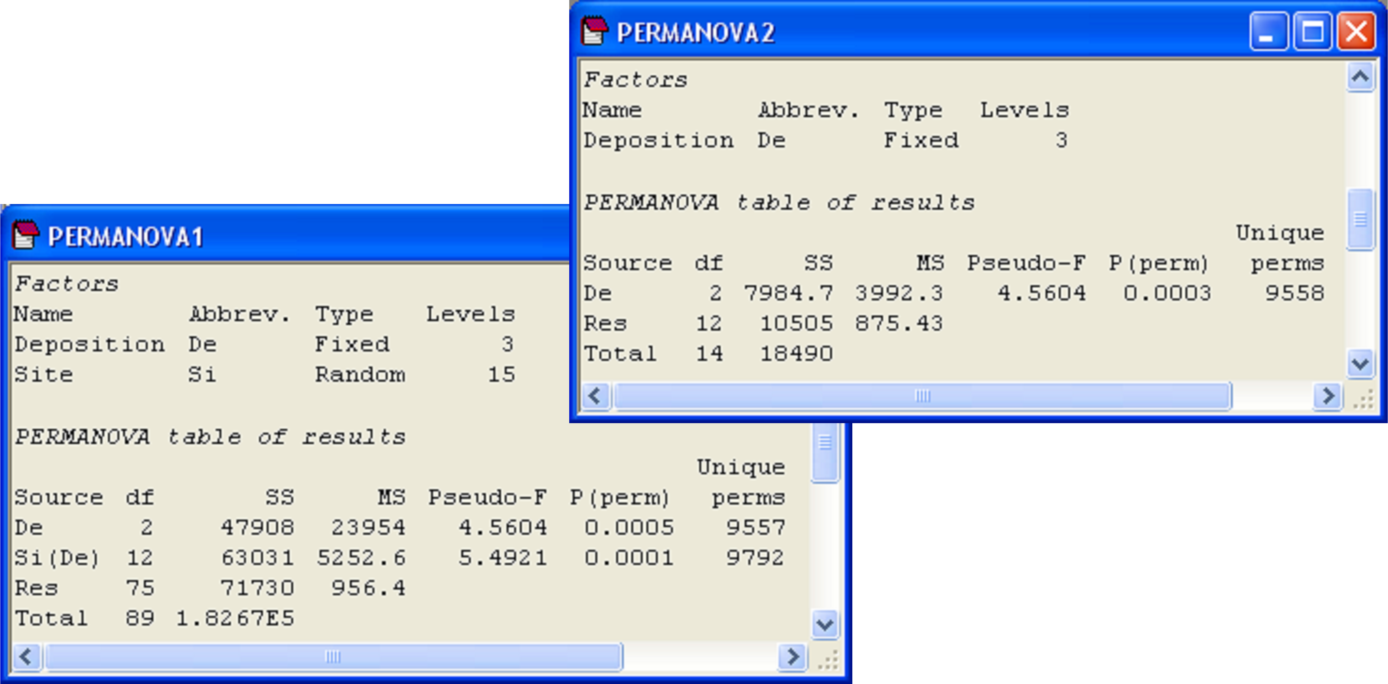Fig. 2.14. PERMANOVA of the Okura data from time 1 according to the two-factor nested design and the test for depositional effects alone in a one-factor design on the basis of resemblances among site centroids.