1.36 Linear combinations of mean squares (NZ fish assemblages)

Several aspects of the above analysis demonstrate its affinity with unbalanced designs. Note that: (i) the multipliers for components of variation in each EMS are not whole numbers; and (ii) the multipliers for a given component of variation are not the same in different EMS’s. As a consequence of these two things, for many of the terms in the model, there is no other single term that, alone, can provide a MS which can act as a denominator to yield a correct pseudo-F ratio. What this generally means for such cases is that some linear combination of mean squares must be used in order to construct a test of the given null hypothesis of interest. Depending on how these linear combinations are constructed, this can also mean that even the degrees of freedom used for the tests are not whole numbers (Fig. 1.49)!

The good news is that the PERMANOVA routine is actually equal to this (rather horrendous) task; (i) it determines the correct EMS’s for every term; (ii) it calculates the correct linear combinations of mean squares required to construct pseudo-F ratios to test each hypothesis; and (iii) it determines the correct distributions of each pseudo-F ratio under each relevant null hypothesis using permutations, producing accurate P-values. The routine is also not bothered by non-integer degrees of freedom. The exchangeable units for a given test (e.g., Anderson & ter Braak (2003) ) are chosen using what might be called a “highest-order term” approach⁴⁶. That is, consider the linear combination of mean squares required for a given test. Of the terms giving rise to those mean squares, the term in the denominator which is of highest order (excluding continuous covariates and the residual) is used to identify exchangeable units for that particular test. For example, the terms whose mean squares are included in the denominator for the pseudo-F ratio test of Location in Fig. 1.49 are: Si(Lo), Ar(Si(Lo)) and Res. The highest-order term (excluding the residual) is Ar(Si(Lo)). Therefore, all replicates within an area will be kept together as a group under permutation and the 16 different areas will be the units permuted for the test of Locations in this design. Importantly, after each permutation, the full pseudo-F ratio is constructed according to the requirements of the numerator and denominator, even if either one or both of these are linear combinations of mean squares.

The need to construct linear combinations of mean squares happens not just in highly complex models with covariates, as described above. It is also (much more commonly) required for certain terms even in many balanced designs, especially multi-way designs involving more than one random factor⁴⁷. For example, consider a study of temperate rocky reef fish assemblages as described by Anderson & Millar (2004) . The study consisted of surveys of fish biodiversity, where abundances of fish species were counted in 10 transects (25 m × 5 m) sampled by SCUBA divers from each of 4 sites in each of 2 habitats at each of 4 locations along the northeast coast of New Zealand. These surveys have been done each year in the austral summer. The data provided in the file fishNZ.pri (located in the folder ‘FishNZ’ in the ‘Examples add-on’ directory) are sums across the 10 transects within each site for each of p = 58 fish species from surveys conducted in each of two years: 2004 and 2005⁴⁸. The experimental design here is:

Factor A:	Year (random with a = 2 levels: 4 = 2004 and 5 = 2005).
Factor B:	Location (random with b = 4 levels: B = Berghan Point, H = Home Point, L = Leigh and A = Hahei).
Factor C:	Habitat (fixed with c = 2 levels: b = urchin-grazed ‘barrens’ and k = kelp forest). 

It is of interest to test the null hypothesis of no difference between the two habitats in fish assemblages. It is also (secondarily) of interest to test and quantify the variability among years and among locations in fish community structure. An analysis of the data according to the above experimental design using PERMANOVA has been done on the basis of the scaled binomial deviance dissimilarity measure (see Anderson & Millar (2004) for a description of this measure), yielding the results shown in Fig. 1.50.

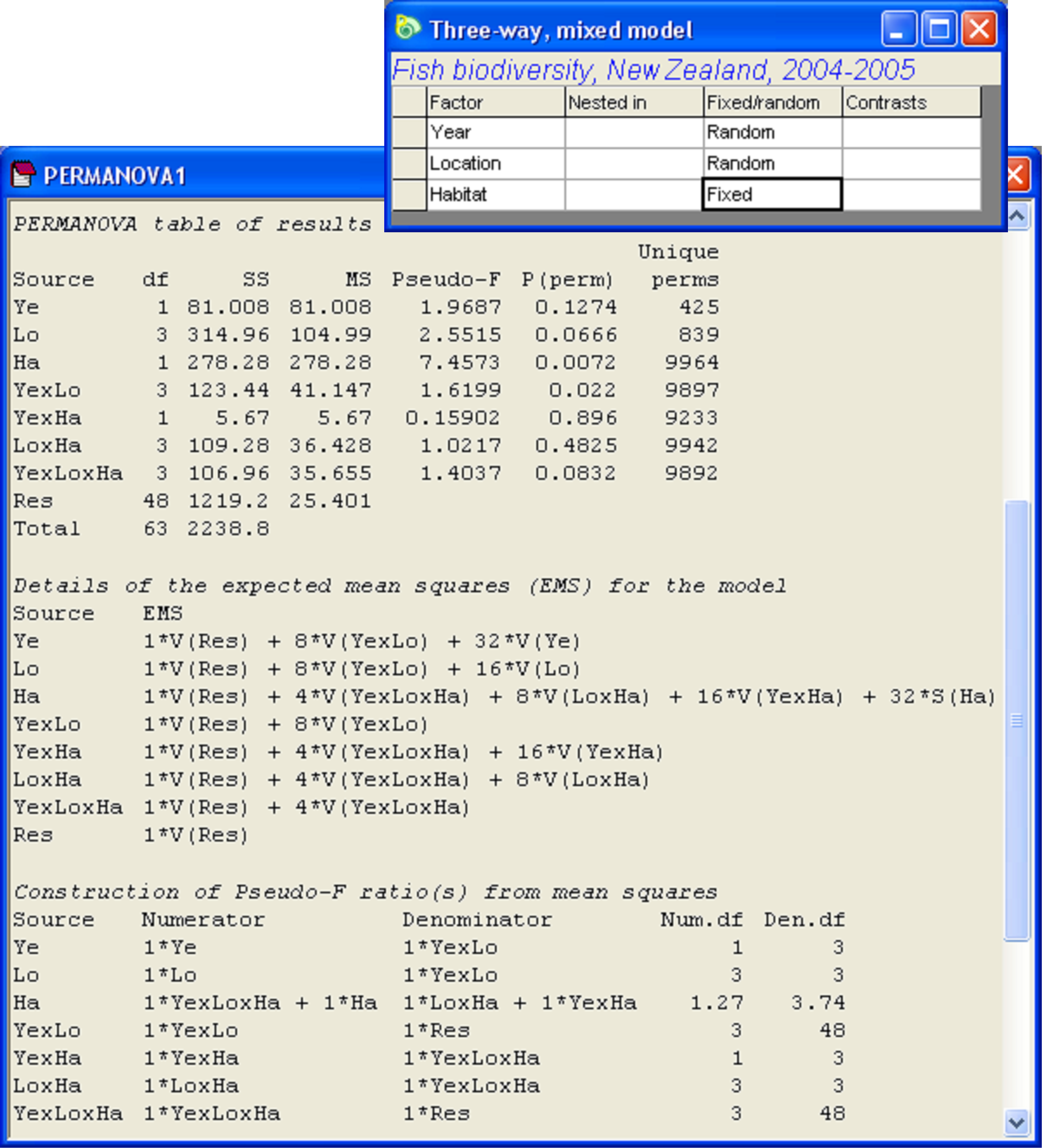
Fig. 1.50. Analysis of New Zealand temperate reef fish according to the three-way mixed model. Note the linear combination of mean squares needed to test the habitat main effect: ‘Ha’.

What is of immediate interest to us here is the test for the main effect of ‘Habitat’ or ‘Ha’ in the output⁴⁹. The EMS for this factor is:

Now, to construct pseudo-F, we need to find a denominator mean square whose expectation is equal to the above when the null hypothesis that S(Ha) = 0 is true. That is, we need a denominator whose expectation is:

However, there is clearly no single term that, alone, can perform this duty, because we require both the Lo×Ha and the Ye×Ha components of variation to appear here. We can see, however, that the term we seek can be obtained by constructing a linear combination of mean squares:

It is desirable, however, not to include mean squares negatively, as this could generate negative pseudo-F ratios, which are not really sensible (e.g., Searle et al. 1992 Searle, Casella & McCulloch (1992) ). Thus, re-arranging the above (so that all mean square terms appear positively), we have:

or

Accordingly, if we wish to construct a pseudo-F ratio where the numerator and denominator will have the same expectation if H$_0$: S(Ha) = 0 is true, and which gets large with increases in the size of S(Ha) alone then we can use:

This is precisely the pseudo-F ratio constructed by the PERMANOVA program, as stated in the results in the line for ‘Ha’ under the heading ‘Construction of Pseudo-F ratio(s) from mean squares’ (Fig. 1.50).

The exchangeable units for this test, using the “highest-order term” approach, are obtained by considering all of the terms involved in the construction of pseudo-F (apart from the term being tested, which is ‘Ha’ here) and determining the one with the highest order. The terms involved are: Ye×Lo×Ha, Ye×Ha and Lo×Ha. The term with the highest order is Ye×Lo×Ha, so the exchangeable units for this test are the a × b × c = 2 × 4 × 2 = 16 cells. So, the n = 4 sites occurring within each of those cells will be permuted together as a unit and the full pseudo-F will be re-constructed after each permutation in order to test the term ‘Ha’ in this case ⁵⁰.

The attentive user will notice the large P-values (> 0.25) associated with a couple of the terms in the model, namely the ‘Ye×Ha’ and ‘Lo×Ha’ interaction terms. If possible, it is desirable to pool (remove) such terms, thereby simplifying the construction of pseudo-F and potentially increasing power (see the section Pooling or excluding terms, above). Only one term should be removed at a time, beginning with the one having the smallest mean square (e.g., Fletcher & Underwood (2002) ), as this will affect the tests and estimated components of variation for other terms in the model. By following this procedure, it is found that ‘Ye×Ha’ and ‘Lo×Ha’ can each be removed (in that order), yielding the results shown in Fig. 1.51. Note that, in this case, after pooling, no linear combinations of mean squares were required for any of the remaining tests.

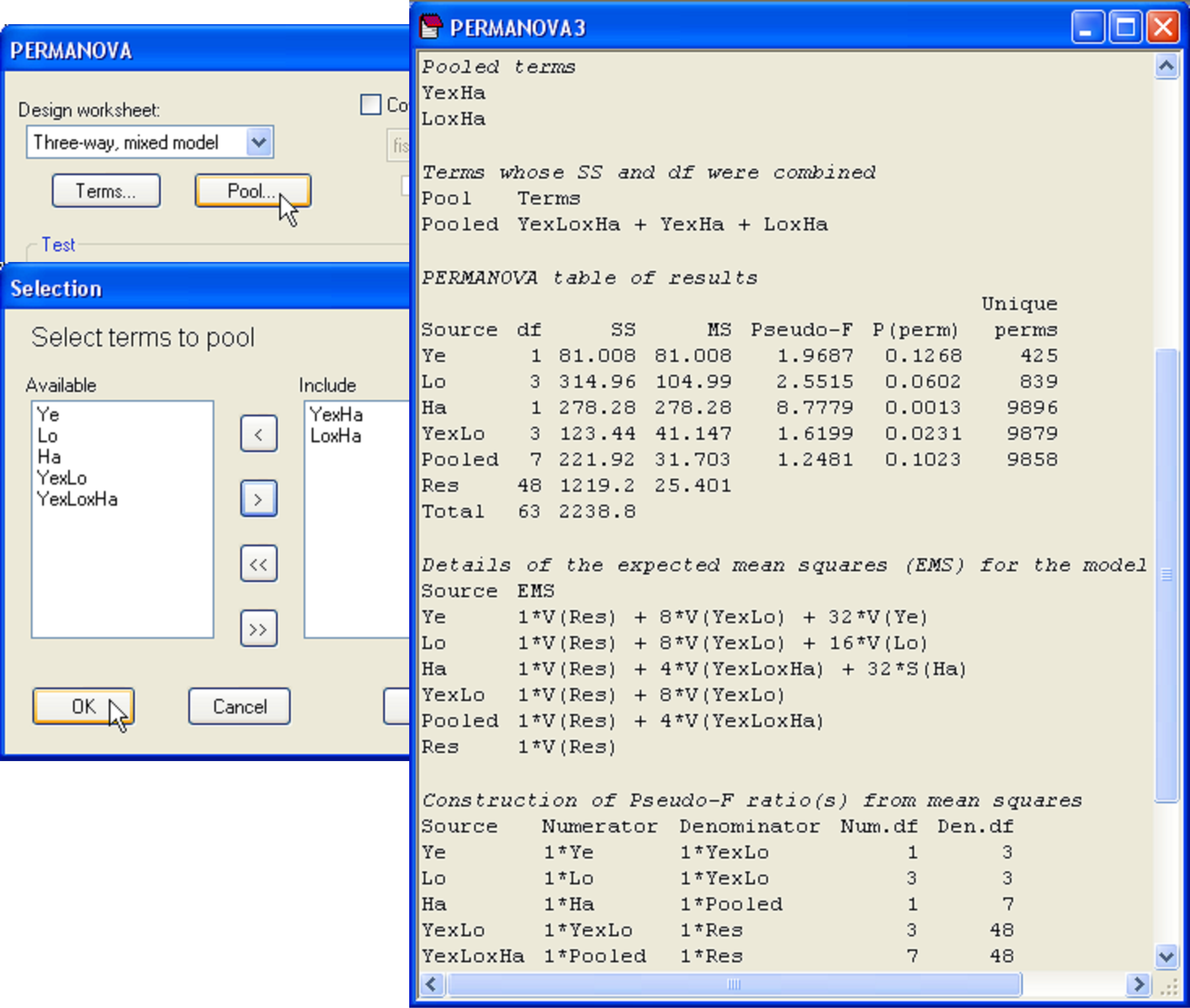
Fig. 1.51. PERMANOVA of the New Zealand fish assemblages after pooling of terms, showing the dialog used at the second step in the pooling procedure, when the term ‘Lo×Ha’ was pooled along with ‘Ye×Ha’, which had previously been pooled at step one.

In traditional univariate ANOVA, the potential use of pooling for these kinds of situations was very important. This is because the construction and subsequent testing of traditional F ratios using linear combinations of mean squares in the numerator and denominator is fraught with difficulties, primarily because ratios of linear combinations of mean squares (called “quasi” F ratios by Quinn & Keough (2002) , see also Blackwell, Brown & Mosteller (1991) ) no longer have (known) F distributions under a true null hypothesis, even when the usual assumptions of normality, homogeneity, etc. are fulfilled (see also Searle, Casella & McCulloch (1992) ). Complicated approximations have therefore been suggested in order to obtain P-values for these cases (e.g., Satterthwaite (1946) , Gaylor & Hopper (1969) ), in the event that pooling was not possible.

One of the most important advantages of the PERMANOVA routine is that it uses permutation tests to obtain P-values. Thus, as long as: (i) the test statistic is constructed correctly in the sense that it isolates the term of interest under the null hypothesis; and (ii) the permutations are done so as to create alternative realisations under a true null hypothesis by permuting appropriate exchangeable units, then the calculations of the P-values are correct and can be used for valid inference. This is true whether or not the corresponding traditional univariate test would be able to be done at all using more traditional theoretical approaches. The more general unified approach of the new PERMANOVA software caters even for these situations (such as the need for linear combinations of mean squares), where the traditional tests would be very difficult (sometimes even impossible) to formulate. Also, of course, PERMANOVA can be implemented on distance or dissimilarity matrices which have been calculated from either univariate or multivariate data.

---

⁴⁶ The order of a term is defined here as follows: a main effect (e.g., A, B, …) is of first order, a two-way interaction (e.g., A×B) is of second order, a three-way interaction (e.g., A×B×C) is of third order, and so on. Also, a nested term, such as B(A), is of second order, while C(A×B) or C(B(A)) would both be of third order, etc.

⁴⁷ The need to use linear combinations of mean squares to construct appropriate pseudo-F statistics will also arise much more commonly (or for more of the terms in the model) if the constraint that fixed effects should sum to zero across levels of random factors in mixed interactions is not applied (i.e., if one chooses to remove the $\checkmark$ in front of the option ‘Fixed effects sum to zero’ in the PERMANOVA dialog).

⁴⁸ Note that these are not the same years as those analysed by Anderson & Millar (2004) , but are data from more recent surveys.

⁴⁹ See the above section Inference space and power regarding the logic and hypotheses underlying tests of fixed main effects even in the presence of potentially non-zero interactions with random factors.

⁵⁰ Although some preliminary simulation work has indicated that this “highest-order term” approach works well in trial cases in terms of maintaining rates of type I error at chosen significance levels, a more complete study of this rather complex issue of appropriate exchangeable units for F ratios involving linear combinations of mean squares would be welcome.