5.8 CAP versus PERMANOVA

It might seem confusing that both CAP and PERMANOVA can be used to test for differences among groups in multivariate space. At the very least, it begs the question: which test should one use routinely? The main difference between these two approaches is that CAP is designed to ask: are there axes in the multivariate space that separate groups? In contrast, PERMANOVA is designed to ask: does between-group variation explain a significant proportion of the total variation in the system as a whole? So, CAP is designed to purposely seek out and find groups, even if the differences occur in obscure directions that are not apparent when one views the data cloud as a whole, whereas PERMANOVA is more designed to test whether it is reasonable to consider the existence of these groups in the first place, given the overall variability. Thus, in many applications, it makes sense to do the PERMANOVA first and, if significant differences are obtained, one might consider then using the CAP analysis to obtain rigorous measures of the distinctiveness of the groups in multivariate space (using cross-validation), to characterise those differences (e.g., by finding variables related to the canonical axes) and possibly to develop a predictive model for use with future data.

One can also consider the difference between these two methods in terms of differences in the role that the data cloud plays in the analysis vis-à-vis the hypothesis¹⁰⁷. For CAP, the hypothesis is virtually a given and the role of the data cloud is to predict that hypothesis (the X matrix plays the role of a response). For PERMANOVA, in contrast, the hypothesis is not a given, and the role of the data cloud is as a response, with the hypothesis (X matrix) playing the role of predictor. This fundamental difference is also apparent when we consider the construction of the among-group SS in PERMANOVA and compare it with the trace statistic in CAP. For PERMANOVA, the among-group SS can be written as tr(HGH) or, equivalently (if there were no negative eigenvalues), we could write: tr(HQH). This is a projection of the variation in the resemblance matrix (represented by Q here) onto the X matrix, via the projection matrix H. For PERMANOVA, all of the PCO axes are utilised and they are each standardised by their eigenvalues ($\lambda$’s, see chapter 3). On the other hand, the trace statistic in CAP is tr(Q$^0 _m$′HQ$^0 _m$). The roles of these two matrices (Q and H) are therefore swapped. Now we have a projection of the X variables (albeit sphericised, since we are using H) into the space of the resemblance matrix instead. Also, the PCO axes in CAP are not scaled by their respective eigenvalues, they are left as orthonormal axes (SS = 1). The purpose of this is really only to save a step. When predicting one set of variables using another, the variables used as predictors are automatically sphericised as part of the analysis¹⁰⁸. Since the eigenvector decomposition of matrix G produces orthonormal PCO axes Q$^0$, we may as well use those directly, rather than multiplying them by their eigenvalues and then subsequently sphericising them, which would yield the same thing!

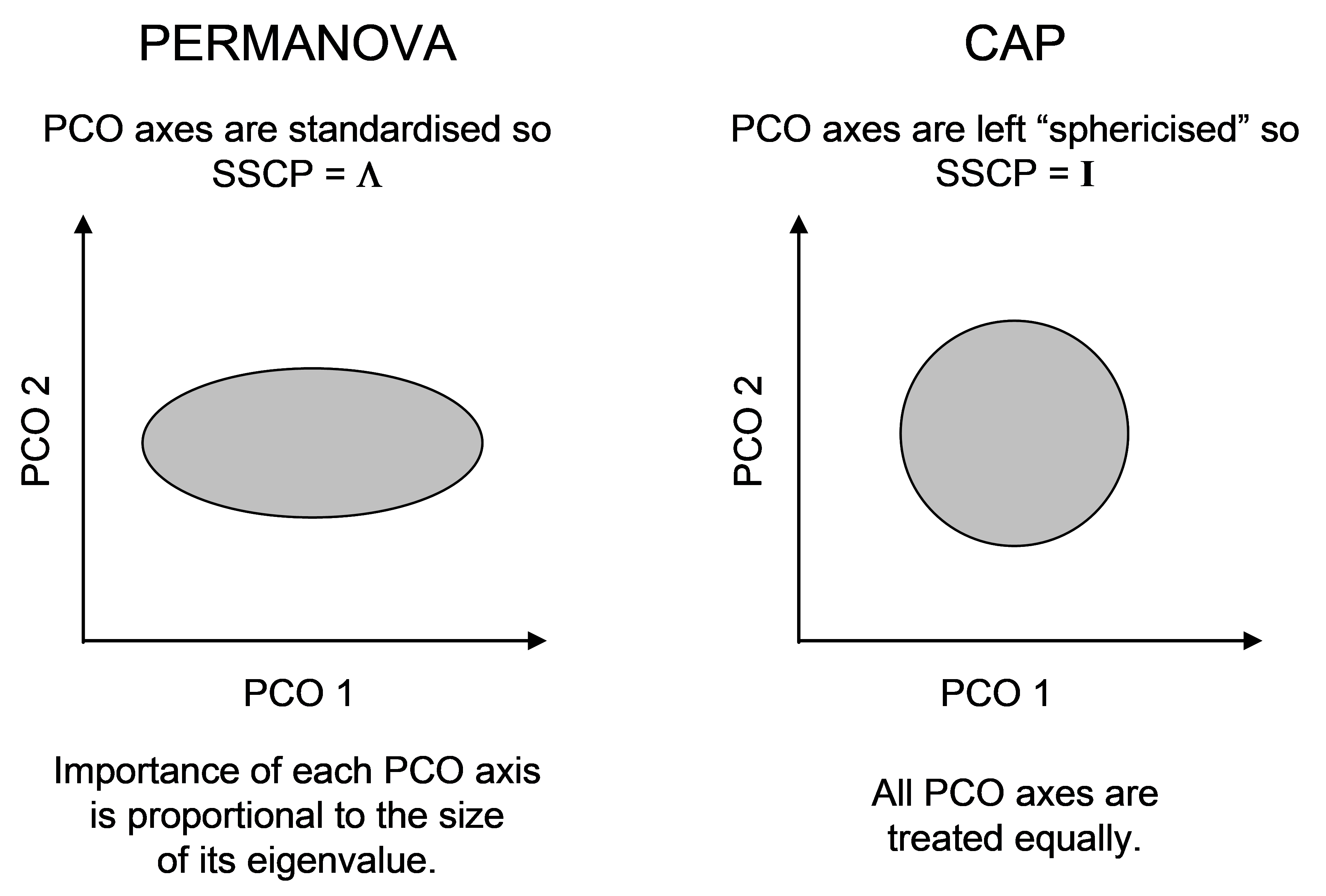Fig. 5.11. Schematic diagram of the difference in the scaling of PCO axes for PERMANOVA vs CAP.

The difference in the scaling of PCO axes, nevertheless, highlights another difference between CAP and PERMANOVA. In PERMANOVA, the relative importance of each PCO axis is in proportion to its eigenvalue (its variance), whereas in CAP, each PCO is given equal weight in the analysis (Fig. 5.11). The latter ensures that directions that otherwise might be of minor importance in the data cloud as a whole, are given equal weight when it comes to searching for groups. This is directly analogous to the situation in multiple regression, where predictor variables are automatically sphericised (normalised to have SS = 1 and rendered independent of one another) when the hat matrix is calculated.

Another way of expressing the ‘sphericising’ being done by CAP is to see its equivalence with the classical MANOVA statistics, where the between-group variance-covariance structure is scaled by a (pooled) within-group variance-covariance matrix (assumed to be homogeneous among groups). The distances between points being worked on by CAP therefore can also be called Mahalanobis distances (e.g., Seber (1984) ) in the multivariate PCO space because they are scaled in this way. In contrast, to obtain the $SS _ A$ of equation (1.3) for PERMANOVA one could calculate the univariate among-group sum of squares separately and independently for each PCO axis and then sum these up¹⁰⁹. Similarly, the $SS _ \text{Res}$ of equation (1.3), may be obtained as the sum of the individual within-group sum of squares calculated separately for each PCO axis. PERMANOVA’s pseudo-F is effectively therefore a ratio of these two sums¹¹⁰.

The relative robustness and power of PERMANOVA versus CAP in a variety of circumstances is certainly an area warranting further research. In terms of performance, we would expect the type I errors for the CAP test statistic and the PERMANOVA test statistic to be the same, as both use permutations to obtain P-values so both will provide an exact test for the one-way case when the null hypothesis is true. However, we would expect the power of these two different approaches to differ. In some limited simulations (some of which are provided by Anderson & Robinson (2003) , and some of which are unpublished), CAP was found to be more powerful to detect effects if they were small in size and occurred in a different direction to the axis of greatest total variation. On the other hand, PERMANOVA was more powerful if there were multiple independent effects for each of a number of otherwise unrelated response variables. Although there is clearly scope for more research in this area, the take-home message must be to distinguish and use these two methods on the basis of their more fundamental conceptual differences (Fig. 5.12), rather than to try both and take results from the one that gives the most desirable outcome!
 

Fig. 5.12. Schematic diagram of the conceptual and practical differences, in matrix algebra terms, between the CAP analyses and PERMANOVA (or DISTLM).

---

¹⁰⁷ The data cloud in the space of the appropriate resemblance measure is represented either by matrix G, Gower’s centred matrix, or by matrix Q, the matrix of principal coordinate axes.

¹⁰⁸ The reader may recall that, for the very same reason, it makes no difference to a dbRDA whether one normalises the X variables before proceeding or not (see chapter 4). The dbRDA coordinate scores and eigenvalues will be the same. Predictor variables are automatically sphericised as part of multiple regression, as a consequence of constructing the H matrix.

¹⁰⁹ Note that the SS from PCO axes corresponding to negative eigenvalues would contribute negatively towards such a sum.

¹¹⁰ Other test statistics could be used. For example, a sum of the individual F ratios obtained from each PCO axis (e.g., Edgington (1995) , which one might call a “stacked” multivariate F statistic), could also be used, rather than the ratio of sums that is PERMANOVA’s pseudo-F.