1.19 Contrasts

In some cases, what is of interest in a particular experimental design is not necessarily the comparisons among all pairs of levels of some factor found to be significant, but rather to compare one or more groups (or levels) together versus one or more other groups. A comparison such as this is called a contrast and is usually logically formulated at the design stage (a priori). Pair-wise comparisons, on the other hand, are generally done after the analysis, so are also sometimes called unplanned or a posteriori comparisons. For example, in the study of the subtidal epibiotic assemblages, we may especially wish to compare a priori the assemblages in the shaded treatment with those occurring in either the open or the procedural control treatments. That is, we would like to contrast group (S) with groups (C, O), effectively treating the latter two treatments together as a single group. Another possible contrast of interest would be the comparison of the procedural control with the open group (i.e., C versus O), as this contrast would identify possible artefacts of the structure used to create shade.

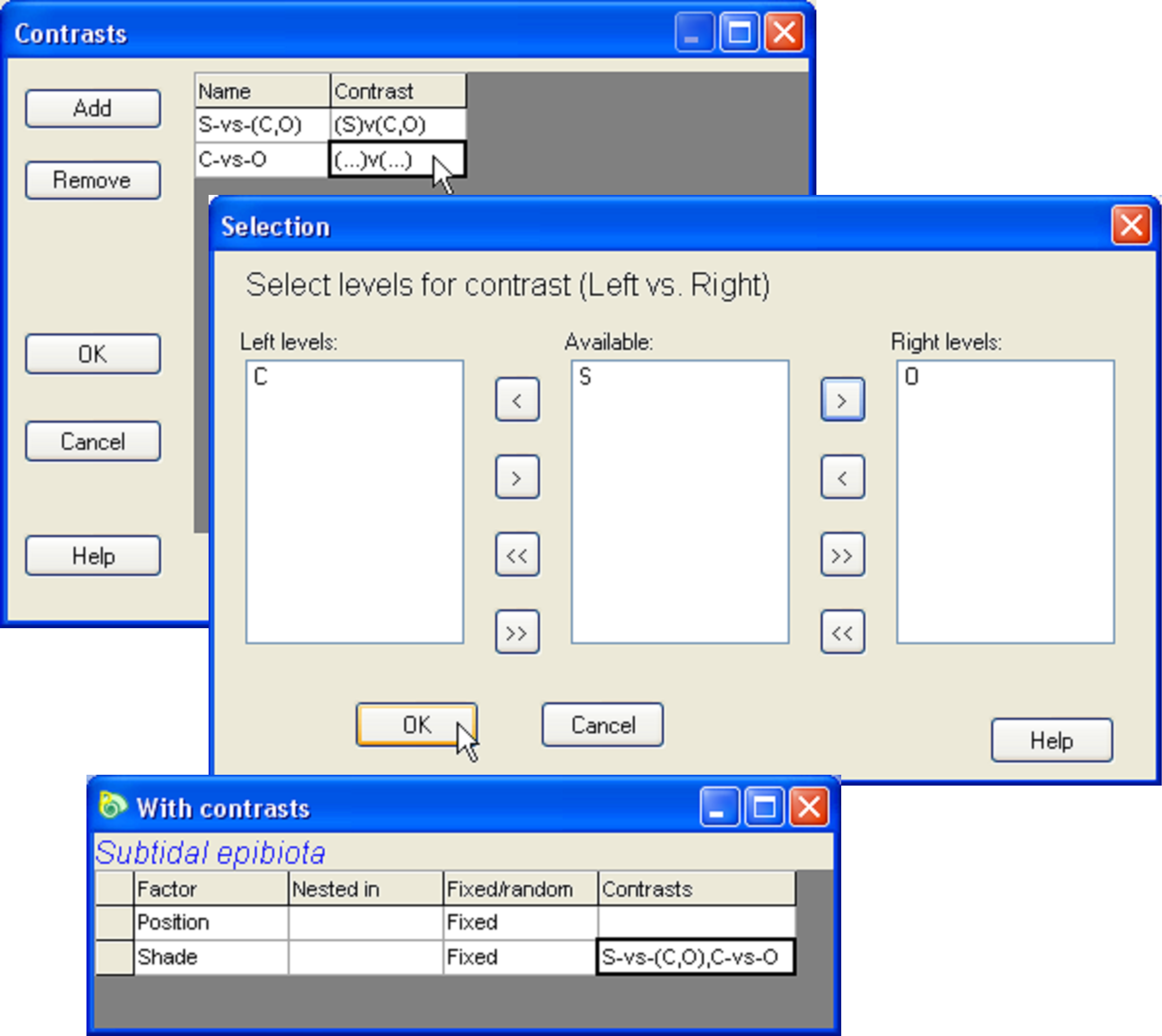Fig. 1.20. Dialog to create contrasts for the subtidal epibiota.

PERMANOVA allows the user to specify particular contrasts of interest. Each of these has 1 degree of freedom and is used to further partition the sums of squares (SS) attributable to that factor. In addition, any interaction terms involving that factor are also partitioned according to the contrast. To see how this works for the subtidal data, click on the design file named Two-way crossed in the sub.pwk workspace and choose Tools>Duplicate, then choose File>Rename Design and name this new design file With Contrasts for reference. Next, in row 2 for the Shade factor, double click on the cell in the final column, headed ‘Contrasts’, which will bring up a new ‘Contrasts’ window (Fig. 1.20). Click on ‘Add’ in order to add a new row to the list of contrasts shown in the window. Double click within the cell in the first column (‘Name’) and type the name S-vs-(C,O). Double click in the cell in the second column (‘Contrast’). This brings up a dialog in which all of the levels available in that factor are listed. Identify the contrast by clicking on S, then on to place it on the left and then click on each of C and O in turn, each followed by , to place the latter two levels on the right, followed by ‘OK’. Next, add a second row in the contrasts window which specifies a contrast of the C and O treatments, to be called C-vs-O (Fig. 1.20). When you are finished, the design file will show the names of the contrasts you have specified in the ‘Contrasts’ column for the Shade factor (Fig. 1.20).

Re-run the PERMANOVA analysis by selecting the resemblance matrix and choosing PERMANOVA+ > PERMANOVA > (Design worksheet: With Contrasts) & (Test $\bullet$Main test) & (Sums of Squares $\bullet$Type III (partial)) & (Permutation method $\bullet$Permutation of residuals under a reduced model) & (Num. permutations: 9999). The contrasts associated with a particular factor are indented in the output file, to emphasise that these are a further partitioning of the SS associated with a given factor (or interactions involving that factor) (Fig. 1.21). These are therefore “extra” tests, in addition to the test of the factor as a whole.

In general, one may construct up to $df _A$ orthogonal (independent) contrasts, where $df _A$ is the number of degrees of freedom for the factor. For these situations (i.e., orthogonal a.k.a. independent contrasts), then the SS for the contrasts chosen will add up to the SS for the factor (that is, if the number of orthogonal contrasts is equal to $df _A$) and it is generally considered unnecessary to worry about doing any corrections for multiple tests. This is true of the example we have done. However, if the contrasts are not orthogonal, and especially if one has chosen to perform a great many contrasts that exceed $df _A$ in number, then the potential inflation of overall type I error due to performing multiple tests may be an issue (see the section on Pair-wise comparisons above).

For our example (Fig. 1.21), the results reveal the strong effect of the shading treatment versus the other two treatments (note how S-vs-(C,O) has a pseudo-F ratio even larger than the pseudo-F for the Shade factor overall) and also show the lack of any apparent procedural artefact (C-vs-O, P = 0.28). In addition, the interaction term of Position × S-vs-(C,O) is approaching statistical significance (P = 0.05), providing increased evidence that the effect of shading (which is tested more directly by this specific contrast than by the test comparing all three treatments) is different near the seafloor compared to far away from the seafloor (e.g., Glasby (1999) ).

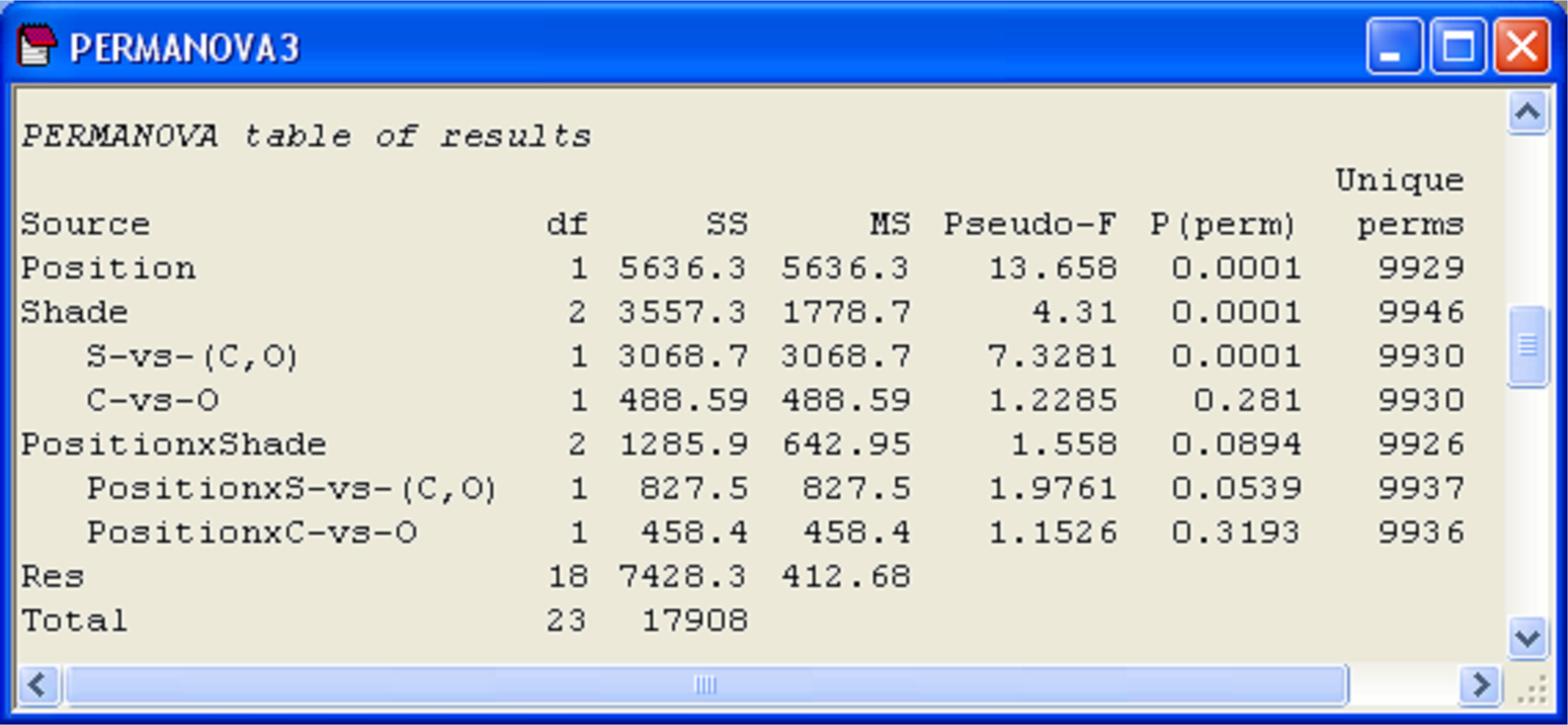Fig. 1.21. Results for subtidal epibiota, including specified contrasts.

A special situation where contrasts might be useful is in the comparison of, say, an impact location versus several control locations in an environmental impact study design ( Underwood (1992) ). If there is no replication of the impact state, but there are several control locations, then this actually generates what is known as an asymmetrical design. For such designs, the correct SS can be obtained using contrasts, however, it is necessary to treat the model explicitly as an asymmetrical design in order to get correct pseudo-F ratios and P-values for all of the tests (see the specific section on Asymmetrical designs below).