4.5 Conditional tests

More generally, when X contains more than one variable, we may also be interested in conditional or partial tests. For example, if X contains two variables X$_1$ and X$_2$, or (more generally) two sets of variables X$_1$ and X$_2$, one may ask: how much of the variation among samples in the resemblance matrix is explained by X$_2$, given that X$_1$ has already been fitted in the model? Usually, the two variables (or sets of variables) are not completely independent of one another, and the degree of correlation between them will result in there being some overlap in the variability that they explain (Fig. 4.5). This means that the amount explained by an individual variable will be different from the amount that it explains after one or more other variables have been fitted. A test of the relationship between a response variable (or multivariate data cloud) and an individual variable alone is called a marginal test, while a test of such a relationship after fitting one or more other variables is called a conditional or partial test. When fitting more than one quantitative variable in a regression-type of context like this, the order of the fit matters.

Fig. 4.5. Schematic diagram of partitioning of variation according to two predictor variables (or sets of variables), X1 and X2.

Suppose we wish to test the relationship between the response data cloud and X$_2$, given X$_1$. The variable(s) in X$_1$ in such a case are also sometimes called covariates⁸⁰. If we consider that the model with both X$_1$ and X$_2$ is called the “full model”, and the model with only X$_1$ is called the “reduced model” (i.e. the model with all terms fitted except the one we are interested in for the conditional test), then the test statistic to use for a conditional test is: $$ F = \frac{ \left( SS _ \text{Full} - SS _ \text{Reduced} \right) / \left( q _ \text{Full} - q _ \text{Reduced} \right) } { \left( SS _ \text{Total} - SS _ \text{Full} \right) / \left( N - q _ \text{Full} - 1 \right) } \tag{4.3} $$ where $SS _ \text{Full}$ and $SS _ \text{Reduced}$ are the explained sum of squares from the full and reduced model regressions, respectively. Also, $q _ \text{Full}$ and $q _ \text{Reduced}$ are the number of variables in X for the full and reduced models, respectively. From Fig. 4.6, it is clear how this statistic isolates only that portion of the variation attributable to the new variable(s) X$_2$ after taking into account what is explained by the other(s) in X$_1$.

Fig. 4.6. Schematic diagram of partitioning of variation according to two sets of predictor variables, as in Fig. 4.5, but here showing the sums of squares used explicitly by the F ratio in equation (4.3) for the conditional test.

The other consideration for the test is how the permutations should be done under a true null hypothesis. This is a little tricky, because we want any potential relationship between the response data cloud and X$_1$ along with any potential relationship between X$_1$ and X$_2$ to remain intact while we “destroy” any relationship between the response data cloud and X$_2$ under a true null hypothesis. Permuting the samples randomly, as we would for the usual regression case, will not really do here, as this approach will destroy all of these relationships⁸¹. What we can do instead is to calculate the residuals of the reduced model (i.e. what is “left over” after fitting X$_1$). By definition, these residuals are independent of X$_1$, and they are therefore exchangeable under a true null hypothesis of no relationship (of the response) with X$_2$. The only other trick is to continue to condition on X$_1$, even under permutation. Thus, with each permutation, we treat the residuals as the response data cloud and calculate pseudo-F as in equation (4.3), in order to ensure that X$_1$ is always taken into account in the analysis. This is required because, interestingly, once we permute the residuals, they will no longer be independent of X$_1$ ( Anderson & Legendre (1999) ; Anderson & Robinson (2001) )! This method of permutation is called permutation of residuals under a reduced model ( Freedman & Lane (1983) ). Anderson & Legendre (1999) showed that this method performed well compared to alternatives in empirical simulations⁸².

The definition of an exact test was given in chapter 1; for a test to be exact, the rate of type I error (probability of rejecting H$_0$ when it is true) must be equal to the significance level (such as $\alpha = 0.05$) that is chosen a priori. Permutation of residuals under a reduced model does not provide an exact test, but it is asymptotically exact – that is, its type I error approaches $\alpha$ with increases in the sample size, N. The reason it is not exact is because we must estimate the relationship between the data cloud and X$_1$ to get the residuals, and this is (necessarily) imperfect – the residuals only approximate the true errors. If we knew the true errors, given X$_1$, then we would have an exact test. Clearly, the estimation gets better the greater the sample size and, as shown by Anderson & Robinson (2001) , permutation of residuals under a reduced model is as close as we can get to this conceptually exact test.

There are (at least) two ways that the outcome of a conditional test can surprise the user, given results seen in marginal tests for individual variables:

• Suppose the marginal test of Y versus X$_2$ is statistically significant. The conditional test of Y versus X$_2$ can be found to be non-significant, after taking into account the relationship between Y and X$_1$.

• Suppose the marginal test of Y versus X$_2$ is not statistically significant. The conditional test of Y versus X$_2$ can be found, nevertheless, to be highly significant, after taking into account the relationship between Y and X$_1$.

The first of these scenarios is somewhat straightforward to visualise, by reference to the graphical representation in Fig. 4.7 (left-hand side). Clearly, if there is a great deal of overlap in the variability of Y explained by X$_1$ and X$_2$, then the fitting of X$_1$ can effectively “wipe-out” a large portion of the variation in Y explained by X$_1$, thus rendering it non-significant. On the other hand, the second of these scenarios is perhaps more perplexing: how can X$_2$ suddenly become important in explaining the variation in Y after fitting X$_1$ if it was originally deemed unimportant when considered alone in the marginal test? The graphical representation in Fig. 4.7 (right-hand side) should help to clarify this scenario: here, although X$_2$ explains only a small portion of the variation in Y on its own, its component nevertheless becomes a significant and substantial proportion of what is left (compared to the residual) once X$_1$ is taken into account. These relationships become more complex with greater numbers of predictor variables (whether considered individually or in sets) and are in fact multi-dimensional, which cannot be easily drawn schematically. The primary take-home message is not to expect the order of the variables being fitted in a sequential model, nor the associated sequential conditional tests, necessarily to reflect the relative importance of the variables shown by the marginal tests.

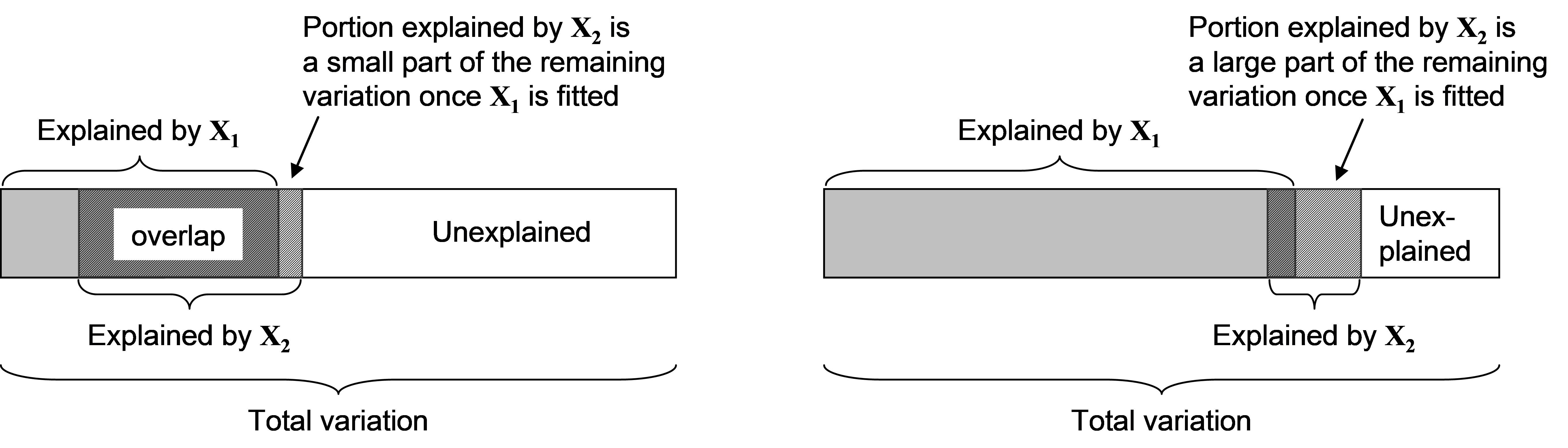
Fig. 4.7. Schematic diagrams showing two scenarios (left and right) where the conditional test of Y versus X$_2$ given X$_1$ can differ substantially from the outcome of the marginal test of Y versus X$_2$ alone.

---

⁸⁰ See also the section entitled Designs with covariates in chapter 1.

⁸¹ But see the discussion in Manly (2006) and also Anderson & Robinson (2001) , who show that this approach can still give reasonable results in some cases, provided there are no outliers in the covariates.

⁸² See the section entitled Methods of permutation in chapter 1 on PERMANOVA for more about permutation of residuals under a reduced model.