5.13 Sphericising variables
It was previously stated that CAP effectively “sphericises” the data clouds as part of the process of searching for inter-correlations between them (e.g., Fig. 5.11). The idea of “sphericising” a set of variables, rendering them orthonormal, deserves a little more attention here, especially in order to clarify further how CAP differs from dbRDA as a method to relate two sets of variables. Let us begin by thinking about a single variable, X. To centre that variable, we would simply subtract its mean. Furthermore, to normalise that variable, we would subtract its mean and divide by its standard deviation. A normalised variable has a mean of zero, a standard deviation of 1 and (therefore) a variance of 1. Often, variables are normalised in order to put them on an “equal footing” prior to multivariate analysis, especially if they are clearly on different scales or are measured in different kinds of units. When we normalise variables individually like this, their correlation structure is, however, ignored.
Now, suppose matrix X has q variables112 that are already centred individually on their means. We might wish to perform a sort of multivariate normalisation in order to standardise them not just for their differing individual variances but also for their correlation (or covariance) structure. In other words, if the original sums-of-squares and cross-products matrix (q × q) for X is:
$$ SSCP _ X = {\bf X ^ \prime X} \tag{5.1} $$
we might like to find a sphericised version of X, denoted X$^ 0$, such that:
$$ SSCP _ {X ^ 0} = {\bf X} ^ {0 \prime} {\bf X} ^ 0 = {\bf I} \tag{5.2} $$
where I is the identity matrix. In other words, the sum of squares (or length, which is the square root of the sum of squares,
Wickens (1995)
) of each of the new variables in X$^ 0$ is equal to 1 and each of the cross products (and hence covariance or correlations between every pair of variables) is equal to zero. In practice, we can find this sphericised matrix by using what is known as the generalised inverse from the singular value decomposition (SVD) of X (e.g.,
Seber (2008)
). More specifically, the matrix X (N × q) can be decomposed into three matrices using SVD, as follows:
$$ {\bf X} = {\bf UWV} ^ \prime \tag{5.3} $$
If N > q (as is generally the case), then U is an (N × q) matrix whose columns contain what are called the left singular vectors, V is a (q × q) matrix whose columns contain what are called the right singular vectors, and W is a (q × q) matrix with eigenvalues (w$_ 1$, w$_ 2$, …, w$_ q$) along the diagonal and zeros elsewhere. The neat thing is, we can now use this in order to construct the generalised inverse of matrix X. For example, to get the inverse of X, defined as X$^ {–1} $ and where X$^ {–1} $X = I, we replace W with its inverse W$^ {–1} $ (which is easy, because W is diagonal, so W$^ {–1} $ is a diagonal matrix with (1/w$_ 1$, 1/w$_ 2$, …, 1/w$_ q$) along the diagonal and zeros elsewhere113) and we get:
$$ {\bf X} ^ {-1} = {\bf UW} ^ {-1} {\bf V} ^ \prime \tag{5.4} $$
Similarly, to get X to the power of zero (i.e., sphericised X), we calculate:
$$ {\bf X} ^ {0} = {\bf UW} ^ {0} {\bf V} ^ \prime \tag{5.5} $$
where W$^ 0$ is I, the identity matrix, a diagonal matrix with 1’s along the diagonal (because for each eigenvalue, we can write w$ ^ 0$ = 1) and zeros elsewhere. Another useful result, which also shows how the hat matrix (whether it is used in dbRDA or in CAP) automatically sphericises the X matrix is:
$$ {\bf H} = {\bf X} ^ {0}{\bf X} ^ {0 \prime} \tag{5.6} $$
If matrix algebra makes you squirm (and don’t worry, you are not alone!), then an actual visual example should help do the trick. Suppose I randomly draw N = 20 samples from a bivariate normal distribution with means of [10, 7], variances of [10, 2] and a covariance of 3. Beginning with a simple scatterplot, we can see a clear positive relationship between these two variables (Fig. 5.23a, the sample correlation here is r = 0.747). Now, each variable can be centred on its mean (Fig. 5.23b), and then the cloud can be sphericised using equation 5.5 (Fig. 5.23c). Clearly, this has resulted in a kind of “ball” of points; the resulting variables (X$ ^ 0$) each now have a mean of zero, a sum of squares of 1 (and hence a length of 1) and a correlation of zero. In summary, sphericising a data cloud to obtain orthonormal axes can be considered as a kind of multivariate normalisation that both standardises the dispersions of individual variables and removes correlation structure among the variables. CAP sphericises both of the data clouds (X and Q) before relating them to one another. Similarly, a classical canonical correlation analysis sphericises both the X and the Y data clouds as part of the analysis.
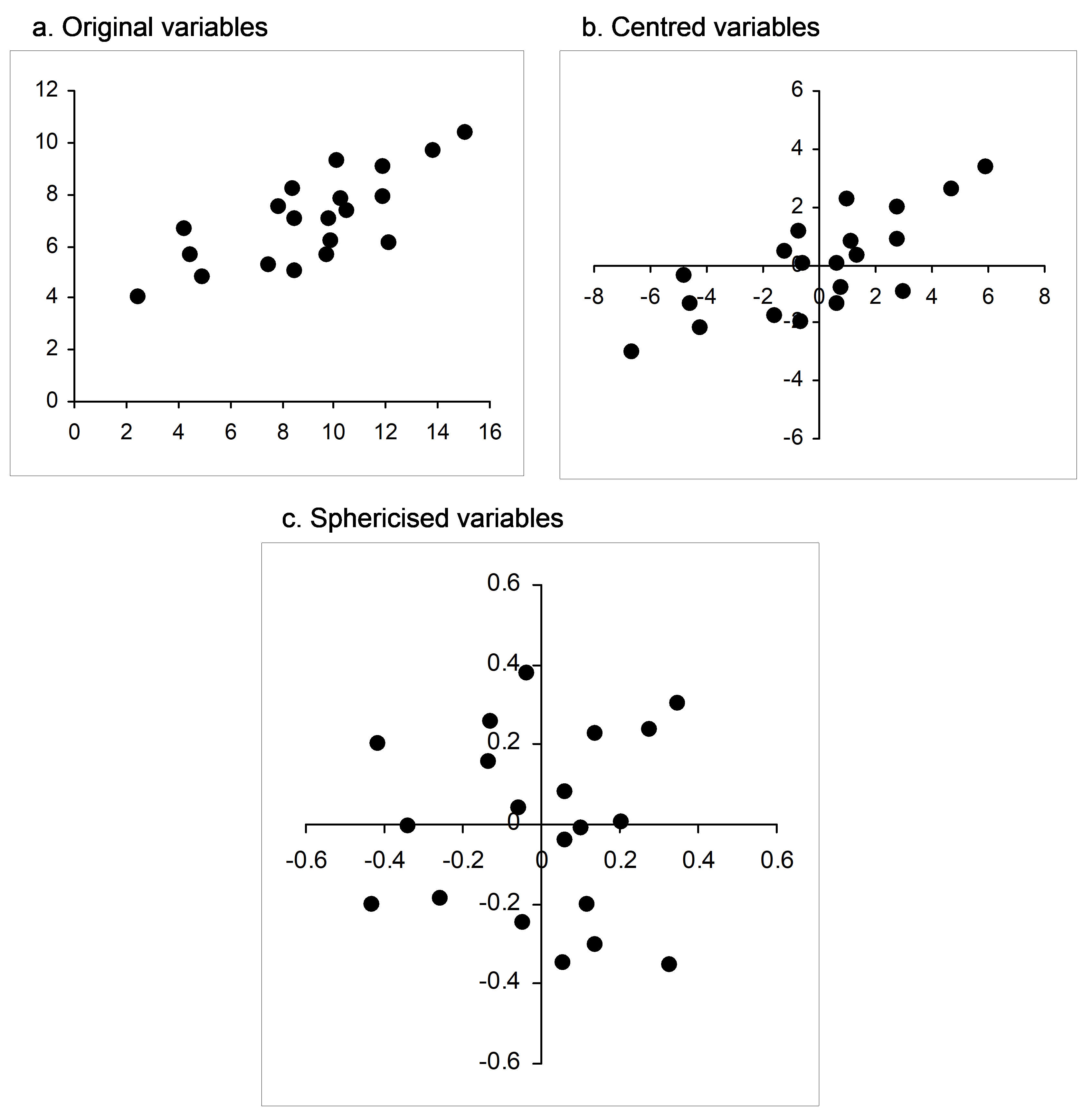 Fig. 5.23. Bivariate scatterplot of normal random variables as (a) raw data, (b) after being centred and (c) after being sphericised (orthonormalised).
112 and suppose also that X is of full rank, so none of the q variables have correlation = 1; all are linearly independent.
113 If X is of full rank, as previously noted, then none of the w eigenvalues in the SVD will be equal to zero. The CAP routine will take care of situations where there are linear dependencies among the X variables (resulting in some of the eigenvalues being equal to zero) appropriately, however, if these are present.