5.10 Adding new samples
A new utility of the windows-based version of the CAP routine in PERMANOVA+ is the ability to place new samples onto the canonical axes of an existing CAP model and (in the case of a discriminant analysis) to classify each of those new samples into one of the existing groups. This is done using only the resemblances between each new sample and the existing set of samples that were used to develop the CAP model. First, these inter-point dissimilarities are used to place the new point onto the (orthonormal) PCO axes. It is then quite straightforward to place these onto the canonical axes, which are simply linear combinations of those PCO axes (see Anderson & Robinson (2003) for more details). The only requirement is that the variables measured on each new sample match the variable list for the existing samples and also that their values occur within the general multivariate region of the data already observed111.
For example, suppose we have three new flowers which we suspect belong to one of the three species of irises analysed by CAP in the section named Test by permutation. Suppose the values of the four morphometric variables for each of these new flowers are:
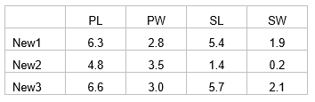
Open the file iris.pri (in ‘Examples add-on\Irises’) and add these three new samples into the data file (use, for example, Edit > Insert > Row), giving them the names of ‘New1’, ‘New2’ and ‘New3’ and typing in the appropriate values for each variable (Fig. 5.14). Choose Edit > Factors and for the factor named ‘Flower’, we clearly do not know which species these three flowers might belong to yet, so give them the level name of ‘New’, to distinguish them from the existing groups of ‘S’, ‘C’ or ‘V’ (Fig. 5.14). One can enter new samples into an existing data file within PRIMER in this fashion, or include the new samples to be read directly into PRIMER with the original data file. The essential criterion for analysis is that the new samples must have a different level name from the existing groups for the factor which is going to be examined in the CAP discriminant analysis. To add new samples to a canonical correlation-type analysis (see below), a factor must be set up which distinguishes the existing samples from new ones (one can use a factor to distinguish ‘model’ samples from ‘validation’ samples, for example).
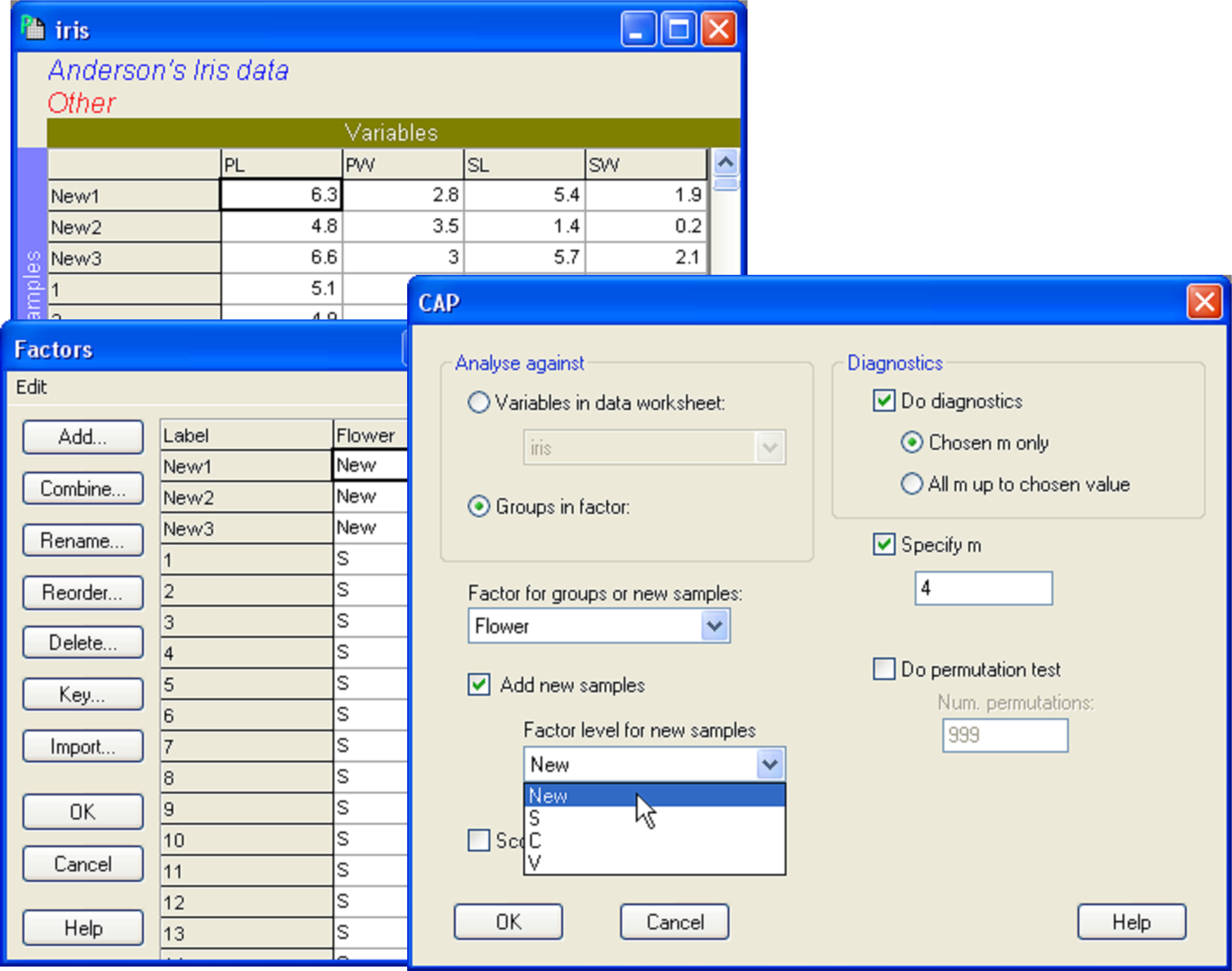 Fig. 5.14. Dialog in CAP showing the addition of three new samples (new individual flowers), to be classified into one of the three species groups using the CAP model developed from the existing data.
Once the new samples have been entered and identified as such, the resemblance matrix for all of the samples together must be calculated. For the iris data set, calculate a Euclidean distance matrix. Proceed with the CAP analysis by choosing: PERMANOVA+ > CAP > (Analyse against •Groups in factor) & (Factor for groups or new samples: Flower) & ($\checkmark$Add new samples > Factor level for new samples New) & (Specify m 4) & (Diagnostics $\checkmark$Do diagnostics •Chosen m only), then click ‘OK’ (Fig. 5.14). The CAP plot shows the three Iris groups, as before, but the new samples are shown using a separate symbol (Fig. 5.15). The only other difference between the CAP plot in Fig. 5.15 compared to Fig. 5.9 is that the y-axis has been flipped. As with PCA, PCO, dbRDA or MDS ordination plots in PRIMER, the signs of the axes are also arbitrary in a CAP plot. The visual representation of the points corresponding to each of the new flowers have been labeled and from this one might make a guess as to which species each of these new samples is likely to belong.
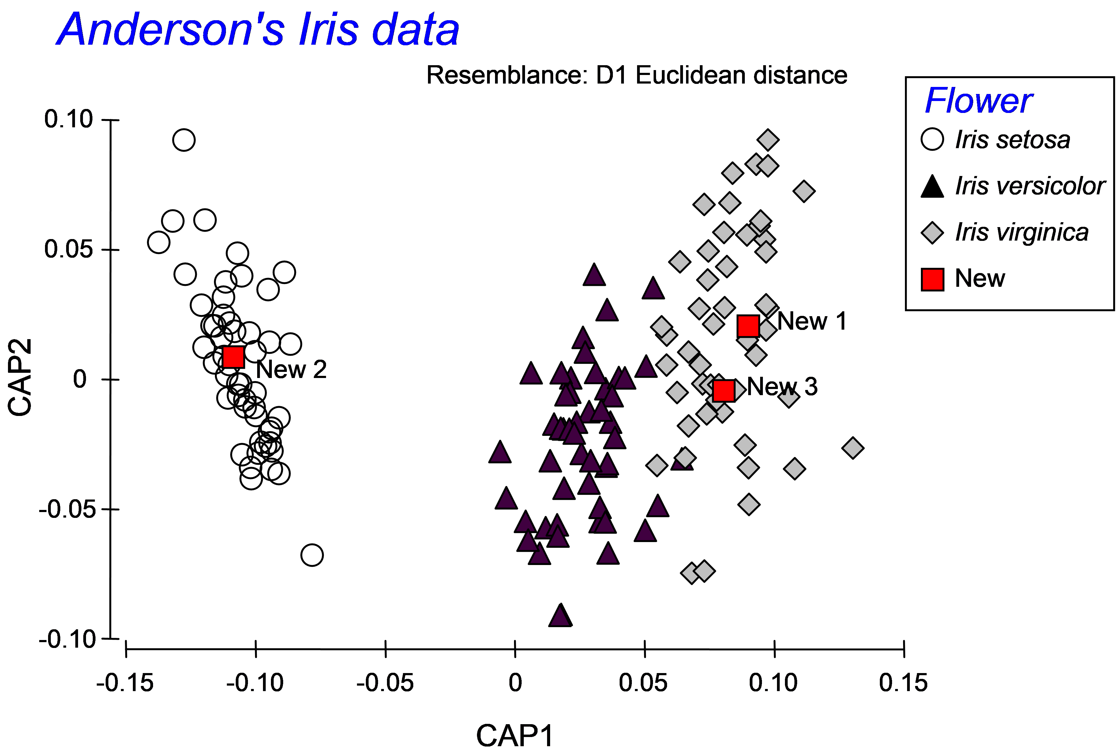 Fig. 5.15. CAP plot of Anderson’s iris data, showing the positions of three new flowers, based on their morphometric resemblances with the other flowers in the existing dataset.
More detailed information is given, however, in the CAP results file under the heading of ‘New samples’ (Fig. 5.16). First are given the positions of each of the new samples on the canonical axes, followed by the classification of each of the new samples according to these positions. In the present case, the samples ‘New1’ and ‘New3’ were allocated to the group Iris virginica, while the sample ‘New2’ was allocated to the group Iris setosa. Each new sample is allocated to the group whose centroid is the closest to it in the canonical space. For reference, the output file includes these distances to centroids for each sample upon which this decision was made (Fig. 5.16).
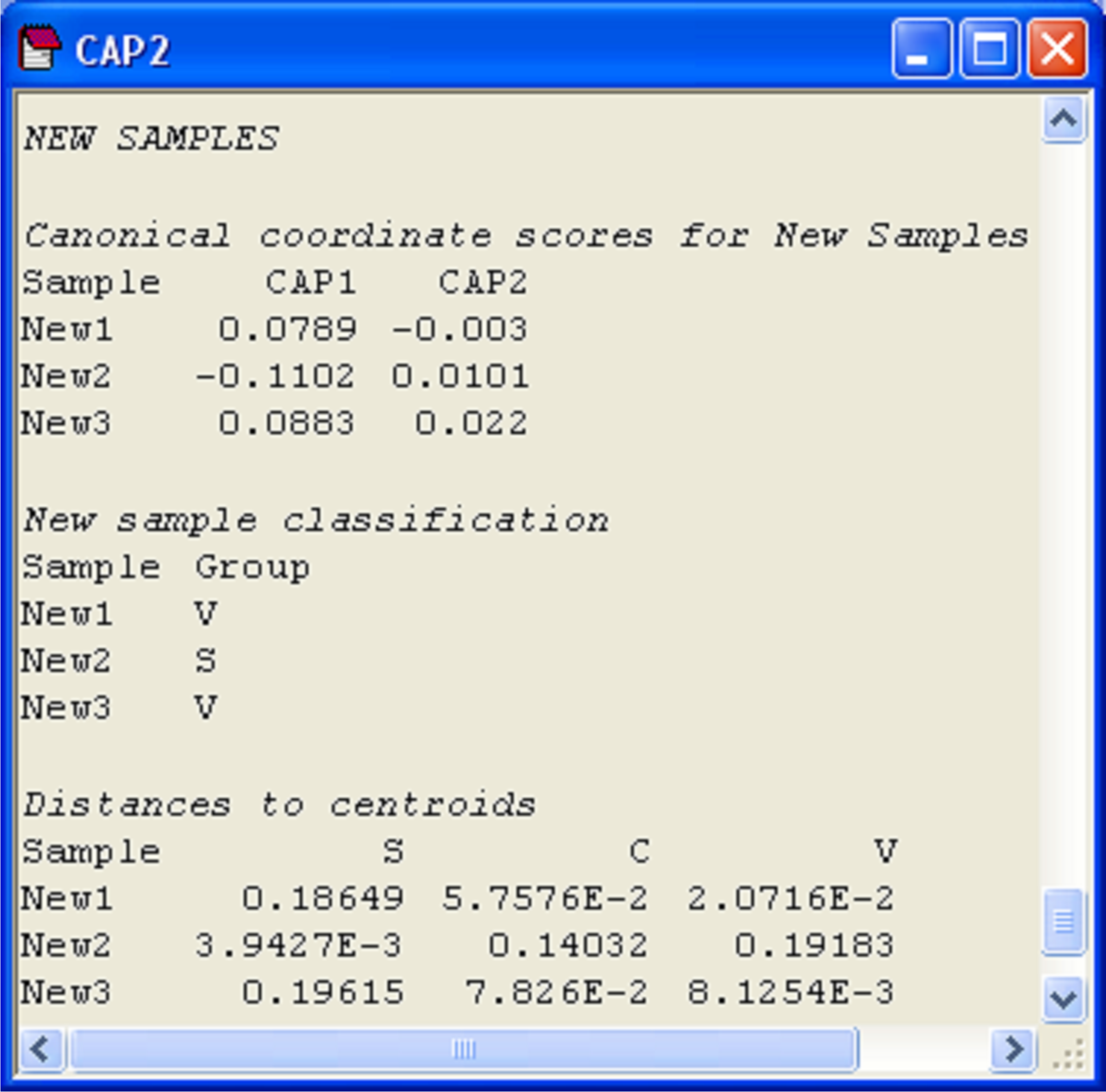 Fig. 5.16. Positions of three new flowers on the canonical coordinate scores, classification of each new flower into one of the groups, and distances from each new flower to each of the group centroids.
111 This latter criterion may be very difficult to check. The CAP routine currently does not attempt to identify data points as “outside previous experience” and the development of an appropriate criterion for doing this would be a worthwhile subject for future research.