1.23 Constructing $F$ from EMS
The determination of the EMS’s gives a direct indication of how the pseudo-F ratio should be constructed in order to isolate the term of interest to test a particular hypothesis (e.g., Table 1.1). Consider the test of the term ‘Block’ (‘Bl’) in the above mixed-model experimental design. The null hypothesis is that there is no significant variability among blocks. Another way of writing this, in the notation used by PERMANOVA, is H$_0$: V(Bl) = 0. To begin, we will construct an F ratio where the numerator is the mean square for the term of interest (e.g., to test blocks, then the numerator will be the mean square for blocks). Now, given the EMS for this numerator term of interest, we essentially need to find a denominator whose expectation would correspond to the numerator if the null hypothesis were true. In the case of the ‘Block’ term, if V(Bl) were equal to zero, then the EMS for blocks would just be 1*V(Res). The term whose EMS corresponds to 1*V(Res) is the residual. Therefore, the pseudo-F ratio for the test of the ‘Block’ term is the mean square for blocks divided by the residual mean square, viz: $F _ {Bl} = MS _ {Bl} / MS _ {Res}$. By following a similar logic, we can see that the test of the interaction term (‘TrxBl’) is provided by $F _ {Tr \times Bl} = MS _ {Tr \times Bl} / MS _ {Res}$ (Table 1.1).
For the ‘Treatment’ term (‘Tr’), we see that its EMS is: 1*V(Res) + 2*V(TrxBl) + 8*S(Tr). The null hypothesis here is that there are no consistent treatment effects, or, equivalently, $ \text{H} _ 0 $: S(Tr) = 0. If the null hypothesis were true, then the EMS for treatments would be: 1*V(Res) + 2*V(TrxBl). The term whose EMS corresponds to this is the interaction term ‘TrxBl’. Therefore, the pseudo-F ratio for the test of no treatment effects is the mean square for treatments divided by the interaction mean square, i.e., $F _ {Tr} = MS_ {Tr} / MS_ {Tr \times Bl}$. Clearly, it would be incorrect to construct $F _ {Tr} = MS_ {Tr} / MS_ {Res}$, because then, if V(TrxBl) were non-zero, we might easily reject $\text{H} _0$: S(Tr) = 0 even if it were true30.
In the PERMANOVA output, the terms which provide the numerator and denominator mean squares for each pseudo-F ratio are provided in the output under the heading ‘Construction of Pseudo-F ratio(s) from mean squares’ (Fig. 1.23). Also given here are the degrees of freedom associated with the numerator (‘Num.df’) and denominator (‘Den.df’) terms. Most of the time, the multipliers on these mean squares will simply be 1, and a single term can be found to provide an appropriate denominator mean square for each of the relevant hypotheses in the model. In some cases, however, a linear combination of mean squares must be sought in order to construct correct pseudo-F ratios to test particular terms (see the section Linear combinations of mean squares). PERMANOVA can deal with these situations and, in such cases, details of the linear combinations used are also provided.
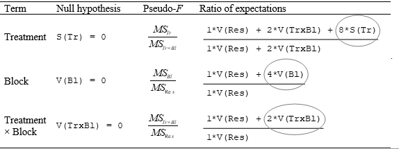
Table 1.1. Null hypothesis, construction of pseudo-F, and ratio of expectations for each term in the mixed model for the study of Tasmanian meiofauna. Note how the construction of pseudo-F isolates the component of interest under the null hypothesis (circled) so that, in each case, the numerator and denominator expectations will match one another if the null hypothesis were true.
30 Some might argue that the existence of an interaction necessarily implies the existence of at least some non-zero treatment effect(s), but we consider the null hypothesis for the test of the main effect in a mixed model such as this to include the concept of consistency in treatment effects, rather than simply the notion of whether there are any treatment effects at all. See the section on Inference space and power.