4.4 Simple linear regression (Clyde macrofauna)

In our first example of DISTLM, we will examine the relationship between the Shannon diversity (H′) of macrofauna and log copper concentration from benthic sampling at 12 sites along the Garroch Head dumpground in the Firth of Clyde, using simple linear regression. How much of the variation in macrofaunal diversity (Y) is explained by variation in the concentration of copper in the sediment (X)? In this case, p = q = 1, so both Y and X are actually just single vectors containing one variable (rather than being whole matrices). We shall do a DISTLM analysis on the basis of Euclidean distances, which is equivalent to univariate simple linear regression, but where the P-value for the test is obtained using permutations, rather than by using traditional tables.

In PRIMER, open up the environmental data file clev.pri and also the macrofaunal data file clma.pri, which are both located in the ‘Clydemac’ folder of the ‘Examples v6’ directory. Here, we will focus first only on a single predictor variable: copper. Highlight the variable ‘Cu’ and choose Select > Highlighted. Next, transform the variable (for consistency, we shall use the log-transformation suggested by Clarke & Gorley (2006) ), by choosing Tools > Transform(individual) > Expression: log(0.1+V). Rename the transformed variable ‘ln Cu’, and also rename the data sheet containing this variable ln Cu. Next, go to the sheet containing the macrofaunal data clma and choose Analyse > DIVERSE. In the resulting dialog, remove the tick marks from all of the measures (shown under the ‘Other’ tab or the ‘Simpson’ tab), so that the only diversity measure that will be calculated is Shannon’s index H′ (shown under the ‘Shannon’ tab) using Log base $\checkmark$e. Place a tick mark next to $\checkmark$Results to worksheet, then click OK. Rename the resulting data sheet H′. Calculate Euclidean distances among samples on the basis of H′ alone. That is, from the H′ data sheet, choose Analyse > Resemblance > (Analyse between •Samples) & (Measure •Euclidean distance).

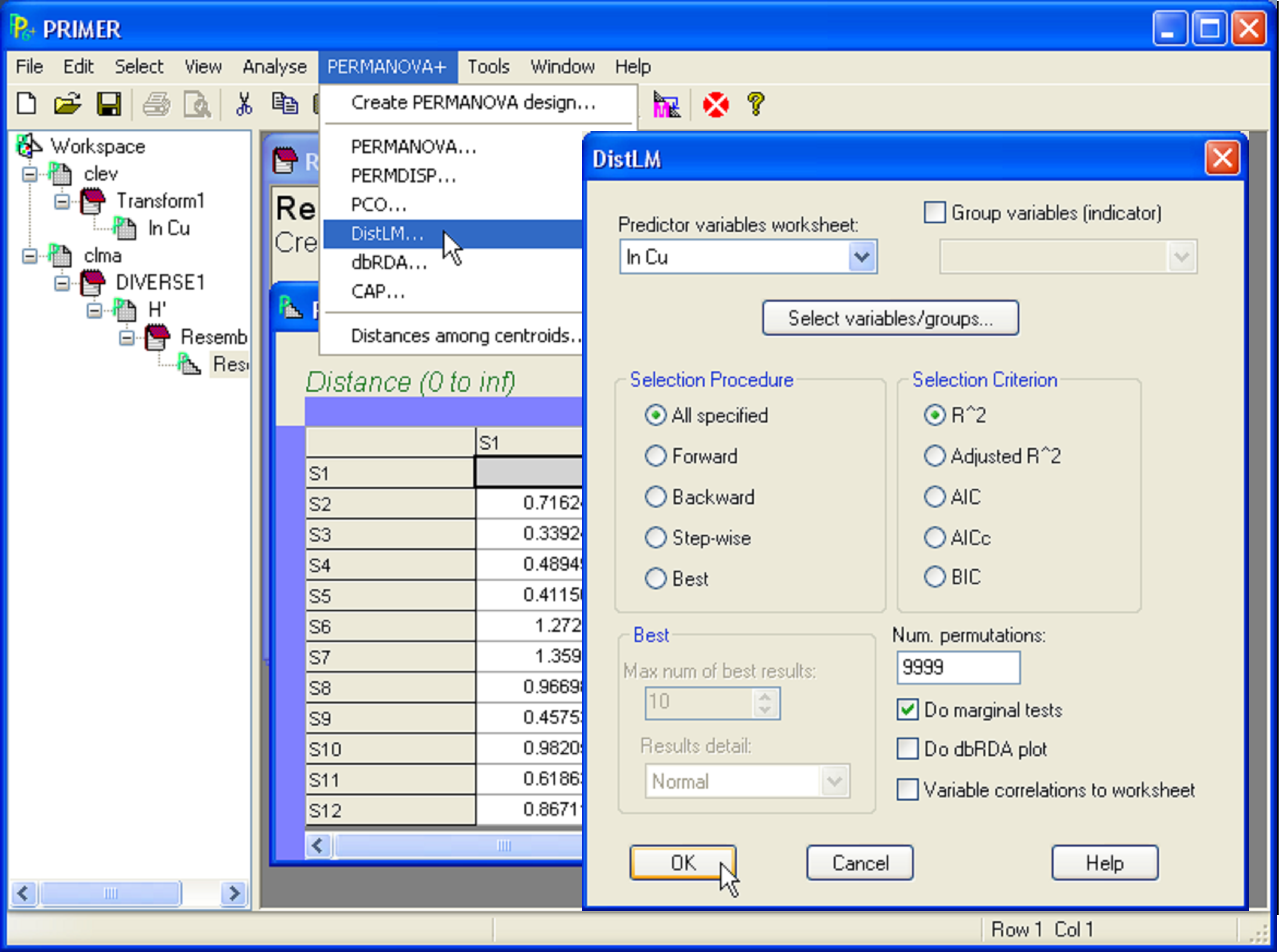
Fig. 4.3. DISTLM procedure for simple linear regression of Clyde macrofaunal diversity (H′) versus log copper concentration (ln Cu).

With the predictor (X) variable(s) in one sheet and the resemblance matrix (arising from the response variable(s) Y) in another, we are now ready to proceed with the analysis. DISTLM, like all of the methods in the PERMANOVA+ add-on, begins from the resemblance matrix. Note that the number and names of the samples in the resemblance matrix have to match precisely the ones listed in the worksheet of predictor variables. They do not necessarily have to be in the same order, but they do have to have the same strict names, so that they can be matched and related to one another directly in the analysis. Choose PERMANOVA+ > DISTLM > (Predictor variables worksheet: ln Cu) & (Selection procedure •All specified) & (Selection criterion •R^2) & (Num. permutations: 9999) (Fig. 4.3).

The results file (Fig. 4.4) shows that the proportion of the variation in Shannon diversity explained by log copper concentrations is quite large ($R ^ 2 = 0.815$, as seen in the column headed ‘Prop.’) and, not surprisingly, statistically significant by permutation (P = 0.0001). Thus, 81.5% of the variation in macrofaunal diversity among these 12 sites (as measured by H′ alone) is explained by variation in log copper concentration. Also shown in the output is the explicit quantitative partitioning: $SS _ \text{Total} = 7.63$ and $SS _ \text{Regression} = 6.22$. As there is only one predictor variable here, the information given under the heading ‘Marginal tests’ (Fig. 4.4) is all that is really needed from the output file. To see a scatterplot for this simple regression case, go to the ln Cu worksheet and choose Tools > Merge > Second worksheet: H′> OK. From this merged data worksheet (called ‘Data1’ by default), choose Analyse > Draftsman Plot > $\checkmark$Correlations to worksheet > OK. The plot shows that H′ decreases strongly with increasing ln Cu and the Pearson linear correlation (r) is -0.903 (Fig. 4.4). Indeed, this checks out with what was given in DISTLM for $R ^2$, as (-0.903)$^2$ = 0.815.

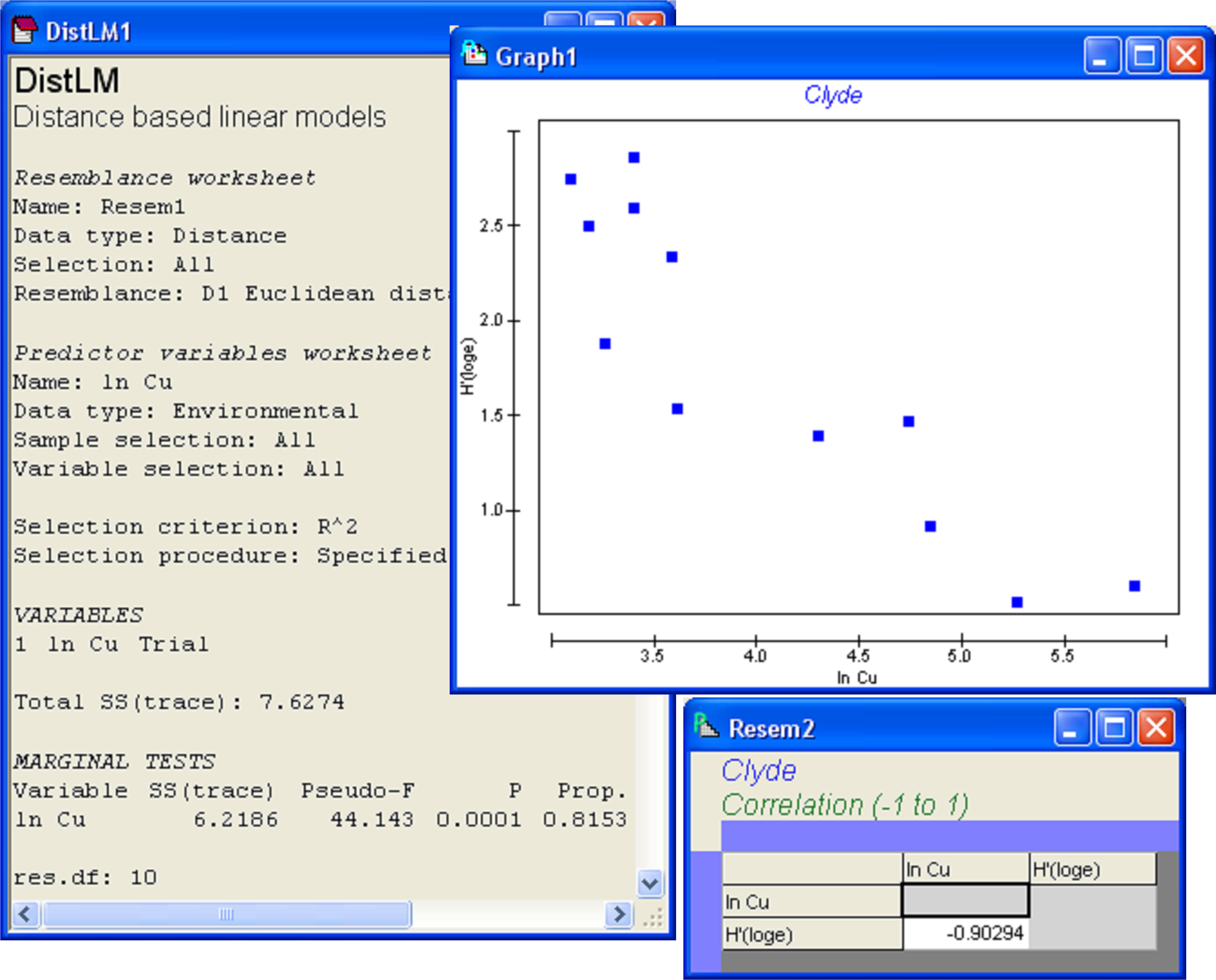
Fig. 4.4. DISTLM results for the regression of diversity of Clyde macrofauna (H′) versus log copper concentration (ln Cu).