4.10 (Ekofisk macrofauna)
We shall now use the DISTLM tool to identify potential parsimonious models for benthic macrofauna near the Ekofisk oil platform in response to several measured environmental variables. The response data (in file ekma.pri in the ‘Ekofisk’ folder of the ‘Examples v6’ directory) consist of abundances of p = 173 species from 3 grab samples at each of N = 39 sites in a 5-spoke radial design (see Fig. 10.6a in Clarke & Warwick (2001) ). Also measured were q = 10 environmental variables (ekev.xls) at each site: Distance (from the oil platform), THC (total hydrocarbons), Redox, % Mud, Phi mean (another grain-size characteristic), and concentrations of several heavy metals: Ba, Sr, Cu, Pb and Ni.
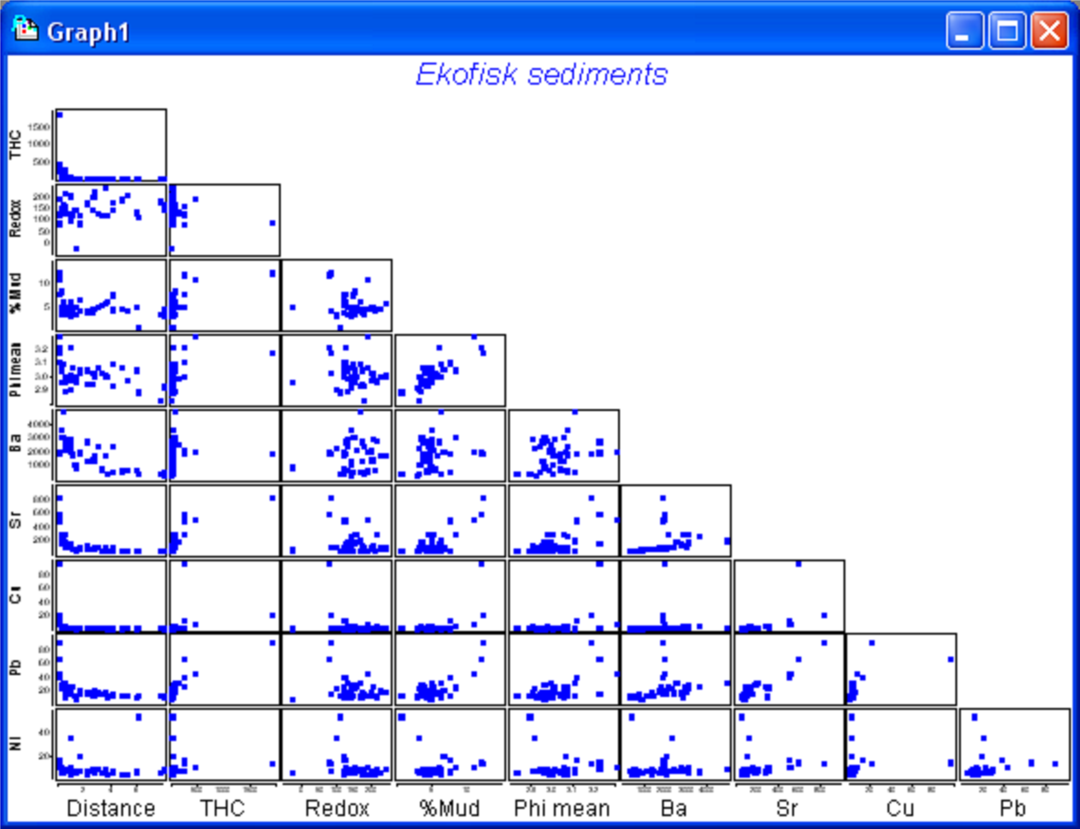
Fig. 4.10. Draftsman plot for the untransformed Ekofisk sediment variables.
We begin by considering some diagnostics for the environmental variables. A draftsman plot indicates that several of the variables show a great deal of right-skewness (Fig. 4.10). The following transformations seemed to do a reasonable job of evening things out: a log transformation for THC, Cu, Pb and Ni, a fourth-root transformation for Distance and % Mud, and a square-root transformation for Ba and Sr. No transformation seems to be necessary for either Redox or Phi mean (Fig. 4.10), the latter already being on a log scale. Transformations were done by highlighting (not selecting) the columns for THC, Cu, Pb and Ni and using Tools > Transform(individual) > (Expression: log(V)) & ($\checkmark$Rename variables). The procedure was then repeated on the resulting data file, first using (Expression: (V)^0.25) on the highlighted columns of Distance and % Mud, and then using (Expression: sqr(V)) on the highlighted columns of Ba and Sr. For future reference, rename the data file containing all of the transformed variables ekevt and save it as ekevt.pri. By choosing Analyse > Draftsman Plot > ($\checkmark$Correlations to worksheet) we are able to examine not just the bivariate distributions of these transformed variables but also their correlation structure (Fig. 4.11).
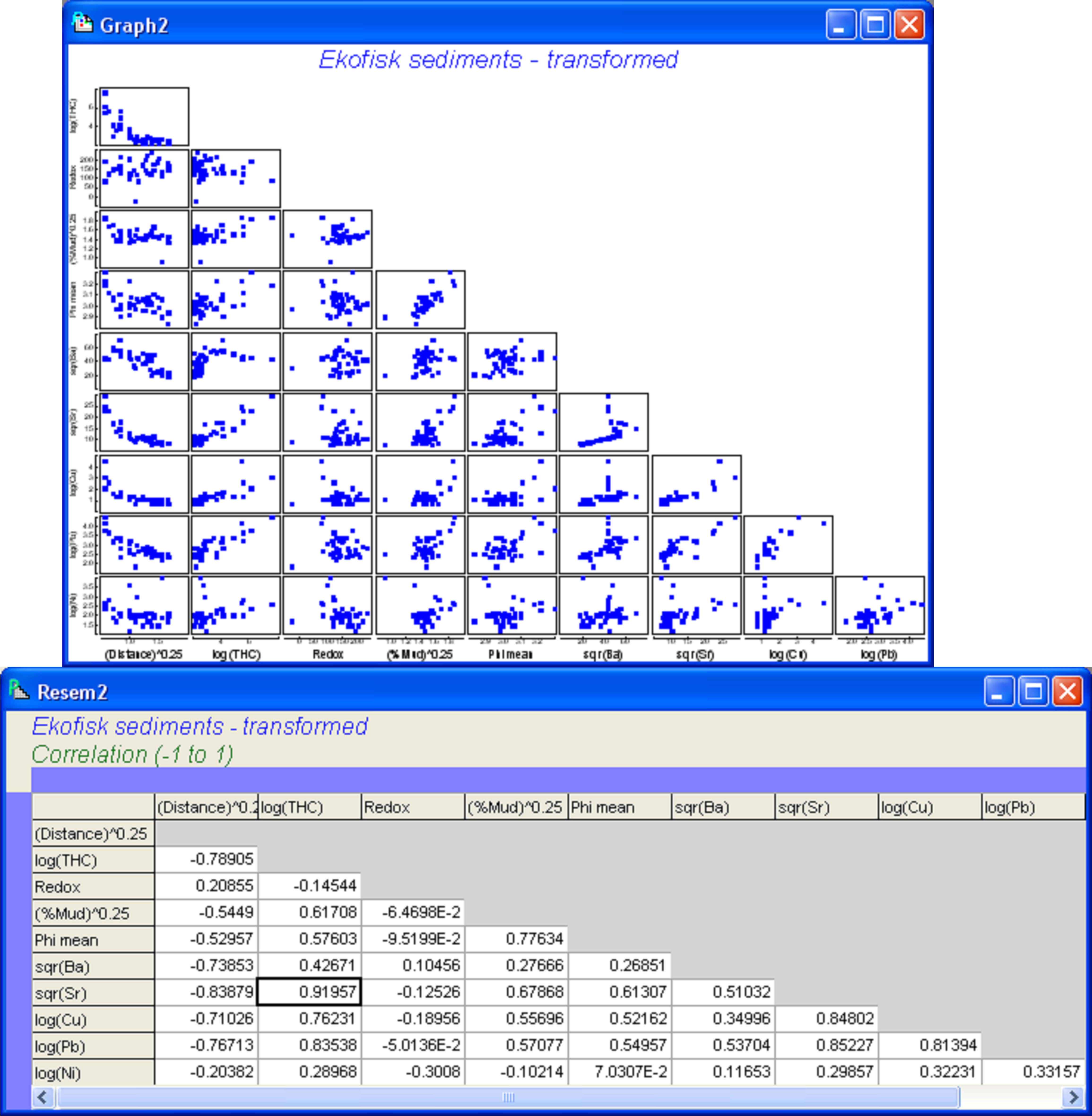
Fig. 4.11. Draftsman plot and correlation matrix for the transformed Ekofisk sediment variables.
For these data, several variables showed strong correlations, such as log(Cu), sqr(Sr) and log(Pb) (|r| > 0.8). The greatest correlation was between sqr(Sr) and log(THC) (|r| = 0.92). These strong inter-correlations provide our first indication that not all of the variables may be needed in a parsimonious model. We may choose to remove one or other of sqr(Sr) or log(THC), as these are effectively redundant variables in the present context. However, their correlation does not quite reach the usual cut-off of 0.95 and it might be interesting to see how the model selection procedures deal with this multi-collinearity. It is worth bearing in mind in what follows that wherever one of these two variables is chosen, then the other could be used instead and would effectively serve the same purpose for modeling.
Note that although the environmental variables may well be on different measurement scales or units, it is not necessary to normalise them prior to running DISTLM, because normalisation is done automatically as part of the matrix algebra of regression (i.e., through the formation of the hat matrix, see Fig. 4.2)87. If we do choose to normalise the predictor variables, this will make no difference whatsoever to the results of DISTLM.
We are now ready to proceed with the analysis of the macrofauna. We shall base the analysis on the Bray-Curtis resemblance measure after square-root transforming the raw abundance values. An MDS plot of these data shows a clear gradient of change in assemblage structure with increasing distance from the oil platform (Fig. 1.7). From the ekma worksheet, choose Analyse > Pre-treatment > Transform (overall) > (Transformation: Square root), then choose Analyse > Resemblance > (Measure •Bray-Curtis). For exploratory purposes, we shall begin by doing a forward selection of the transformed environmental variables, using the R$^2$ criterion. This will allow us to take a look at the marginal tests and also to see how much of the variation in the macrofaunal data cloud (based on Bray-Curtis) all of the environmetal variables, taken together, can explain. From the resemblance matrix, choose PERMANOVA+ > DISTLM > (Predictor variables worksheet: ekevt) & (Selection Procedure •Forward) & (Selection Criterion •R^2) & ($\checkmark$Do marginal tests) & (Num. permutations: 9999).
In the marginal tests, we can see that every individual variable, except for Redox and log(Ni), has a significant relationship with the species-derived multivariate data cloud, when considered alone and ignoring all other variables (P < 0.001, Fig. 4.12). What is also clear is that the variable (Distance)^(0.25) alone explains nearly 25% of the variability in the data cloud, and other variables (sqr(Sr), log(Cu) and log(Pb)) also individually explain substantial portions (close to 20% or more) of the variation in community structure (Fig. 4.12). For the forward selection based on R$^2$, it follows that (Distance)^(0.25) must be chosen first. Once this term is in the model, the variable that increases the R$^2$ criterion the most when added is log(Cu). Together, these first two variables explain 34.4% of the variability in the data cloud (shown in the column headed ‘Cumul.’). Next, given these two variables in the model, the next-best variable to add in order to increase R$^2$ is sqr(Ba), which adds a further 4.17% to the explained variation (shown in the column headed ‘Prop.’). The forward selection procedure continues, also doing conditional tests at each step along the way, until no further increases in R$^2$ are possible. As we have chosen to use raw R$^2$ as our criterion, this eventually simply leads to all of the variables being included. The total variation explained by all 10 environmental variables is 52.2%, a figure which is given at the bottom of the ‘Cumul.’ column for the sequential tests, and which is also given directly under the heading ‘Best solution’ in the output file (Fig. 4.12).
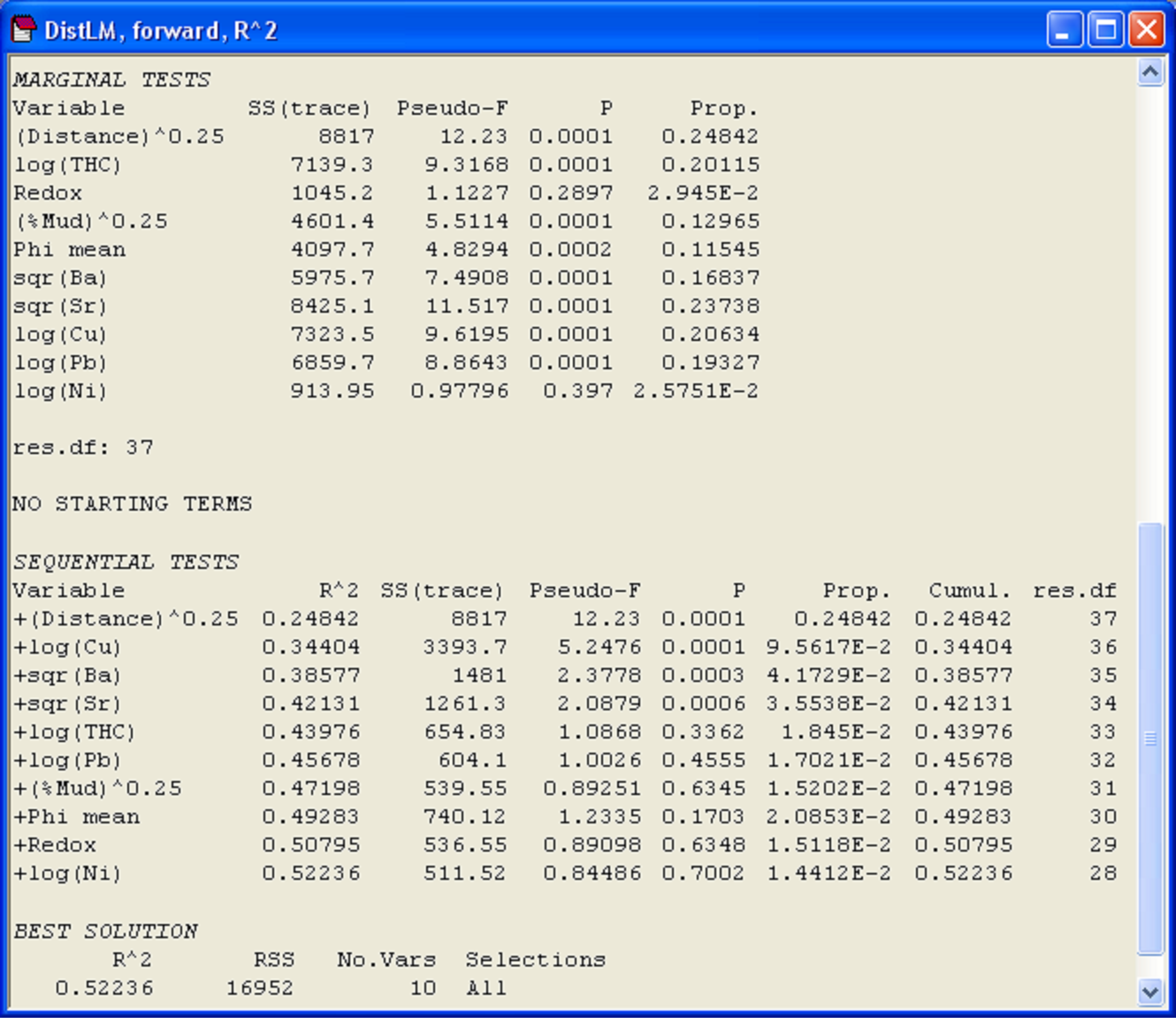
Fig. 4.12. Results of DISTLM for Ekofisk macrofauna using forward selection of transformed environmental sediment variables.
A notable aspect of the sequential tests is that after fitting the first four variables: (Distance)^(0.25), log(Cu), sqr(Ba) and sqr(Sr), the P-value associated with the conditional test to add log(THC) to the model is not statistically significant and is quite large (P = 0.336). There is probably no real further mileage to be gained, therefore, by including log(THC) or any of the other subsequently fitted terms in the model. The first four variables together explain 42.1% of the variation in community structure, and subsequent variables add very little to this (only about 1.5-2% each). Given that we had noticed earlier a very strong correlation between log(THC) and sqr(Sr), it is not surprising that the addition of log(THC) is not really worthwhile after sqr(Sr) is already in the model. Although all of the P-values for this and the subsequent conditional tests are reasonably large (P > 0.17 in all cases), the conditional P-values in forward selection do not necessarily continue to increase and, indeed, a “significant” P-value can crop up even after a large one has been encountered in the list. It turns out that little meaning can be drawn from P-values for individual terms (whether large or small) after the first large P-value has been encountered in a series of sequential tests, as the inclusion of a non-significant term in the model such as this will affect subsequent results in various unpredictable ways, depending on the degree of inter-correlations among the variables.
Based on the forward selection results, we might consider constructing and using a model with these first four chosen variables only. This is clearly a more parsimonious model than using all 10 variables. However, the forward selection procedure is not necessarily guaranteed to find the best possible model for a given number of variables. We shall therefore explore some alternative possible parsimonious models using the AIC and BIC criteria, in turn. From the resemblance matrix, choose PERMANOVA+ > DISTLM > (Predictor variables worksheet: ekevt) & (Selection Procedure •Best) & (Selection Criterion •AIC) & (Best > (Max num of best results: 10) & (Results detail: Normal) ). There is no need to do the marginal tests again, so remove the $\checkmark$ from this option.
When the ‘Best’ selection procedure is used, there are two primary sections of interest in the output. The first is entitled ‘Best result for each number of variables’ (Fig. 4.13). For example, in the present case, the best single variable for modelling the species data cloud is identified as variable 1, which is (Distance)^(0.25). The best 2-variable model, interestingly, does not include variable 1, but instead includes variables 6 and 7, corresponding to sqr(Ba) and sqr(Sr), respectively. The best 4-variable model has the variables numbered 1 and 6-8, which correspond to (Distance)^(0.25), sqr(Ba), sqr(Sr) and log(Cu). Note that the best 4-variable model is not quite the same as the 4-variable model that was found using forward selection, although these two models have values for R$^2$ that are very close. Actually, it turns out that it doesn’t matter which selection criterion you choose to use (R$^2$, adjusted R$^2$, AIC, AIC$_c$ or BIC), this first section of results in the output from a ‘Best’ selection procedure will be identical. This is because, for a given number of predictor variables, the ‘penalty’ term being used within any of these criteria will be identical, so all that will distinguish models having the same number of predictor variables will be the value of $SS _ \text{Residual}$ or, equivalently, R$^2$.
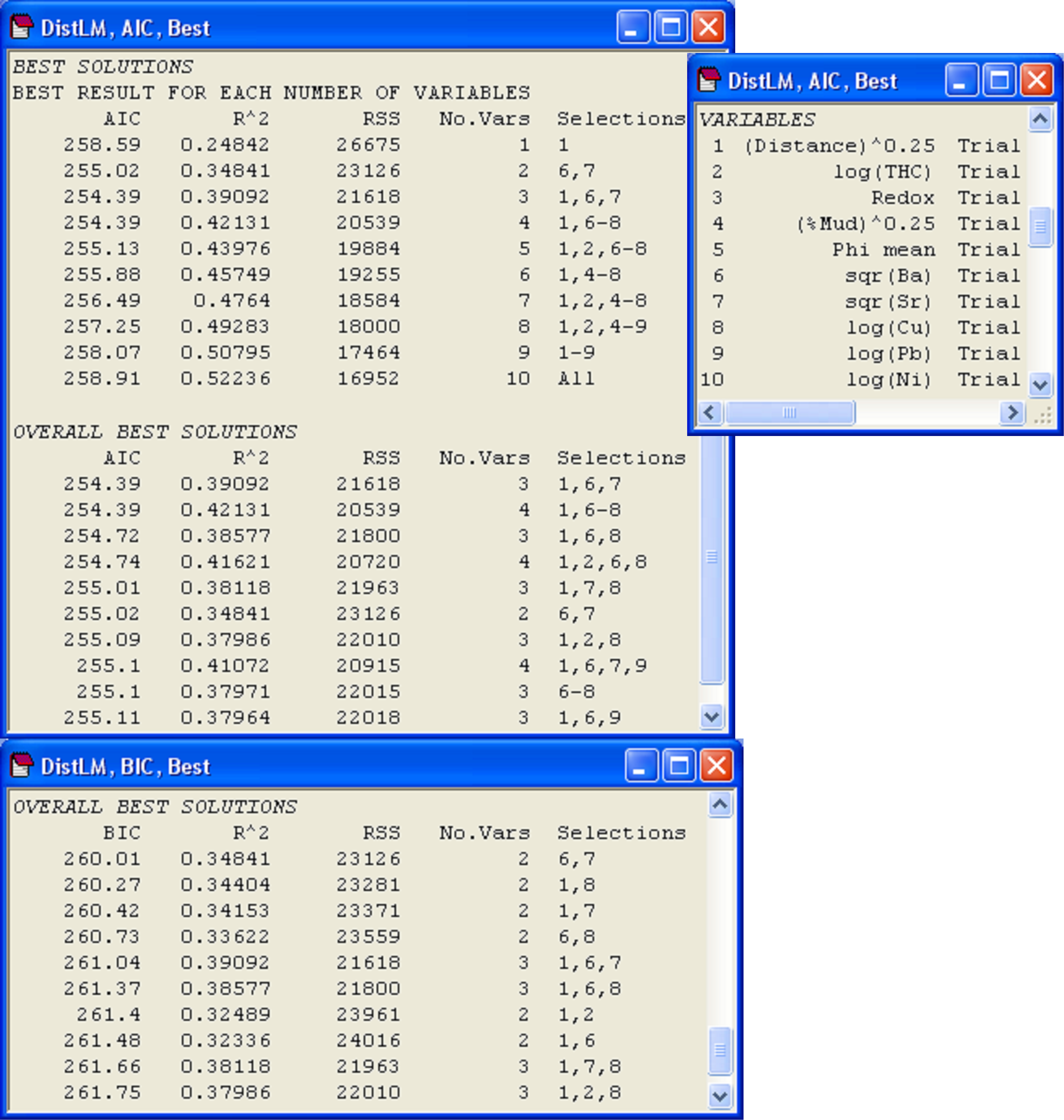
Fig. 4.13. Results of DISTLM for Ekofisk macrofauna using the ‘Best’ selection procedure on the basis of the AIC selection criterion and then (below this) on the basis of the BIC selection criterion.
The next section of results is entitled ‘Overall best solutions’, and this provides the 10 best overall models that were found using the AIC criterion (Fig. 4.13). The number of ‘best’ overall models and the amount of detail provided in the output can be changed in the DISTLM dialog. For the Ekofisk data, the model that achieved the lowest value of AIC (and therefore was the best model on the basis of this criterion) had three variables: 1, 6 and 7 (i.e., (Distance)^(0.25), sqr(Ba) and sqr(Sr) ). Another model that achieved an equally low value for AIC had 4 variables: 1, 6-8. Indeed, a rather large number of models having 3 or 4 variables achieved an AIC value that was within 1 unit of the best overall model, and even one of the 2-variable models (6, 7) was within this range. Burnham & Anderson (2002) (page 131), suggested that models having AIC values within 2 units of the best model should be examined more closely to see if they differ from the best model by 1 parameter while still having essentially the same value for the first (non-penalty) term in equation (4.6). In such cases, the larger model is not really competitive, but only appears to be “close” because it adds a parameter and is therefore within 2 units of the best model (2 $\nu$ = 2 where $\nu$ = 1), even though the fit (as measured by the first term in equation 4.6) is not genuinely improved. Generally, when a number of models produce quite similar AIC values (within 1 to 2 units of each other, as seen here), this certainly suggests that there is a reasonable amount of redundancy among the variables in X, so whichever model is eventually settled on, it is likely that a number of different combinations of predictor variables could be used inter-changeably in order to explain the observed relationship, due to these inter-correlations.
For comparison, we can also perform the ‘Best’ selection procedure using the BIC criterion (Fig. 4.13). The more “severe” nature of the BIC criterion is apparent straight away, as many of the best overall solutions contain only 2 or 3 variables, rather than 3 or 4, as were obtained using AIC. However, a few of the models listed in the top 10 using BIC coincide with those listed using AIC, including {6, 7}, {1, 6, 7}, {1, 6, 8}, {1, 7, 8} and {1, 2, 8}. To achieve a balance between the more severe BIC criterion and the more generous AIC criterion, we could output the top, say, 20 models for each and then examine a scatter-plot of the two criteria for these models. This has been done for the Ekofisk data (Fig. 4.14). An astute choice of symbols (one being hollow and larger than the other) makes it easy to identify the models that appeared in both lists. Note that from the AIC list, it is easy to calculate the BIC criterion (and vice versa), as $SS _ \text{Residual}$ (denoted ‘RSS’ in the output file) and the number of variables in the model (which is $\nu$ – 1) are provided for each model in the list.
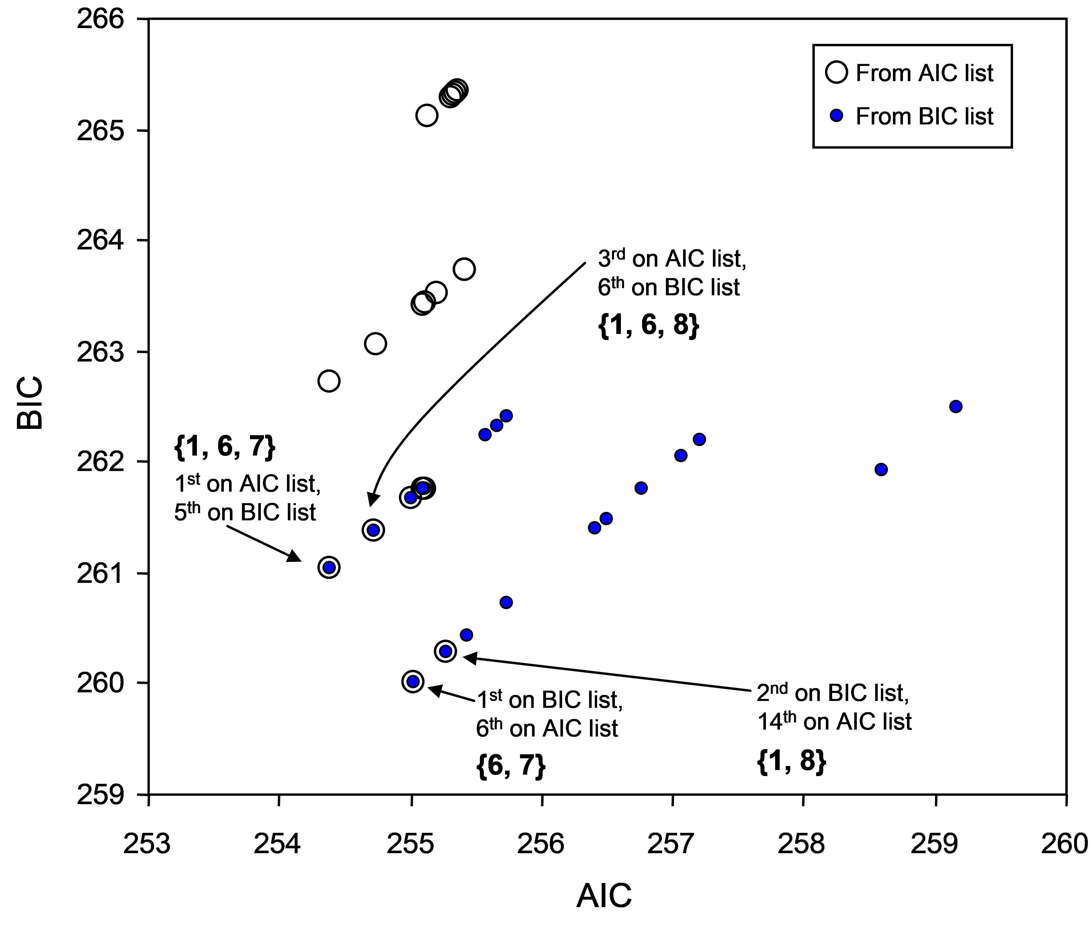 Fig. 4.14. Scatterplot of the AIC and BIC values for each of the top twenty models on the basis of either the AIC criterion or on the basis of the BIC criterion. Some of these models overlap (i.e. were chosen by both criteria).
The exact correlation between AIC and BIC for models having a given number of variables is evident in the scatter plot, as individual models occur along a series of parallel lines (Fig. 4.14). These lines correspond to models having 1 variable, 2 variables, 3 variables, and so on. In this example, most of the best models have 2, 3 or 4 variables. The greatest overlap in models that were listed in the top 20 using either the AIC or BIC criterion occurred for 3-variable models. Moreover, the plot suggests that any of the following models would probably be reasonable parsimonious choices here: {1, 6, 7}, {6, 7} or {1, 6, 8}. Balancing “severity” with “generosity”, we might choose for the time being to use the 3-variable model (bowing to AIC) which had the lowest BIC criterion, i.e., model {1, 6, 7}: (Distance)^(0.25), sqr(Ba) and sqr(Sr), which together explained nearly 40% of the variability in macrofaunal community structure. In making a choice such as this, it is important to bear in mind the caveats articulated earlier with respect to multi-collinearity and to refrain from making any direct causative inferences for these particular variables.
87 This contrasts with the use of the RELATE or BEST procedures in PRIMER, which would require normalisation prior to analysis for situations such as this.