1.33 Unbalanced designs
Virtually all of the examples thus far have involved the analysis of what are known as balanced experimental designs. For these situations, there is equal replication within each level of a factor (or within each cell). Even data that lack replication have an equal number of n = 1 within each cell. However, despite a researcher’s best efforts, sometimes the design ends up being unbalanced, where there are unequal numbers of replicate samples within each factor level (or within each cell) of the design.
For the one-way case (such as the Ekofisk oil-field data seen in the section One-way example), the consequences of an unbalanced design are not problematic. We can perform PERMANOVA in the usual way, with the usual partitioning of sums of squared dissimilarities. Only two consequences of unequal replication are apparent for one-way designs. First, the multiplier on the EMS for the factor of interest is no longer necessarily a whole number, as it was for the balanced case. By scrolling down the PERMANOVA results window produced in the analysis of the Ekofisk oil-field data (shown only partially in Fig. 1.10 above), we can see the multiplier for the ‘S(Di)’ component of variation in the EMS for Distance is 9.57, whereas for any of the balanced designs, the multipliers for any component in any EMS are whole numbers (e.g., see the EMS in Figs. 1.15, 1.23 or 1.29, all of which are balanced designs). For one-way designs, this does not change, however, the use of the residual MS in the denominator of the pseudo-F ratio for the test of “No differences among the groups”.
The second consequence of an unbalanced design is apparent when we consider the permutations. We still randomly allocate observation units across the groups (levels of the factor), while maintaining the existing group differences in sample sizes. Each individual unit no longer has an equal chance of falling into any particular group, but instead will have a greater chance of falling into a group that has a larger sample size. However, we can still proceed easily on the basis that all possible re-arrangements of the samples by reference to the existing (albeit unbalanced) experimental design are equally likely.
The more important issues facing experimenters with unbalanced designs occur when there is more than one factor in the design. In that case, the consequences are: (i) the multipliers on individual components of variation in the EMS’s are not necessarily whole numbers and these multipliers can differ for the same component when it appears in the EMS’s of different terms in the model; (ii) the main effects of factors and the interaction terms are no longer independent of one another. The latter is perhaps the most important conceptual issue in the analysis of unbalanced, as opposed to balanced, designs. This means that, like in multiple regression (see chapter 4), the order in which we choose to fit the terms matters.
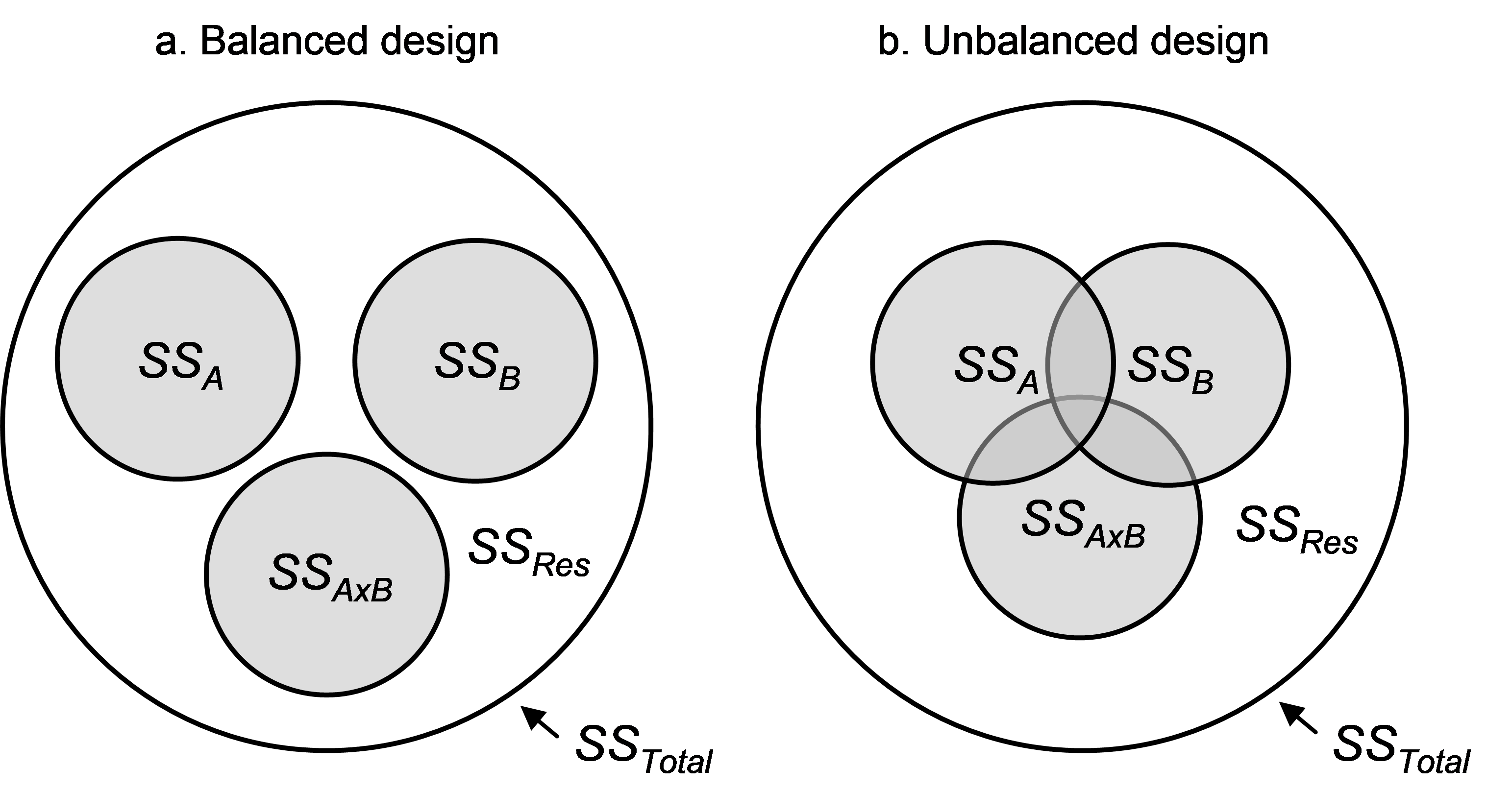
Fig. 1.40. Venn diagrams showing the difference between (a) a balanced and (b) an unbalanced two-way crossed design.
Begin by considering a two-way crossed ANOVA design, with factors A, B and their interaction A×B. If the design is balanced, then the individual amounts of variation in the response data cloud explained by each of the terms in the model are completely independent of one another. This can be visualised using a Venn diagram (Fig. 1.40), where the total variation in the system ($SS _T$) is represented by a large circle and the residual variation, $SS _ {Res}$, is the area left over after removing all of the portions explained by the model. For a balanced design, the individual terms in the model explain separate independent portions of the total variation (Fig. 1.40a), whereas for an unbalanced design, there will be some overlap among the terms regarding the individual portions of variation that they explain (Fig. 1.40b).