3.8 Distances among centroids (Okura macrofauna)

In chapter 1, the difficulty in calculating centroids for non-Euclidean resemblance measures was discussed (see the section entitled Huygens’ theorem). In chapter 2, the section entitled Generalisation to dissimilarities indicated how PCO axes could be used in order to calculate distances from individual points to their group centroids in the space of a chosen resemblance measure as part of the PERMDISP routine. Furthermore (see the section entitled Dispersion in nested designs in chapter 2), it was shown how a new tool available in PERMANOVA+ can be used to calculate distances among centroids in the space of a chosen resemblance measure. One important use of this tool is to provide insights into the relative sizes and directions of effects in complex experimental designs. Specifically, once distances among centroids from the cells or combinations of levels of an experimental design have been calculated, these can be visualised using PCO (or MDS). The results will provide a suitable visual complement to the output given in PERMANOVA regarding the relative sizes of components of variation in the experimental design and will also clarify the relative distances among centroids for individual levels of factors.

For example, we shall consider again the data on macrofauna from the Okura estuary ( Anderson, Ford, Feary et al. (2004) ), found in the file okura.pri of the ‘Okura’ folder in the ‘Examples add-on’ directory. Previously, we considered only the first time of sampling. Now, however, we shall consider the full data set, which included 6 times of sampling. The full experimental design included four factors:

• Factor A: Season (fixed with a = 3 levels: winter/spring (W.S), spring/summer (S.S) or late summer (L.S)).

• Factor B: Rain.Dry (fixed with b = 2 levels: after rain (R) or after a dry period (D)).

• Factor C: Deposition (fixed with c = 3 levels: high (H), medium (M) or low (L) probability of sediment deposition).

• Factor D: Site (random wih d = 5 levels, nested in the factor Deposition).

There were n = 6 sediment cores collected at each site at each time of sampling.

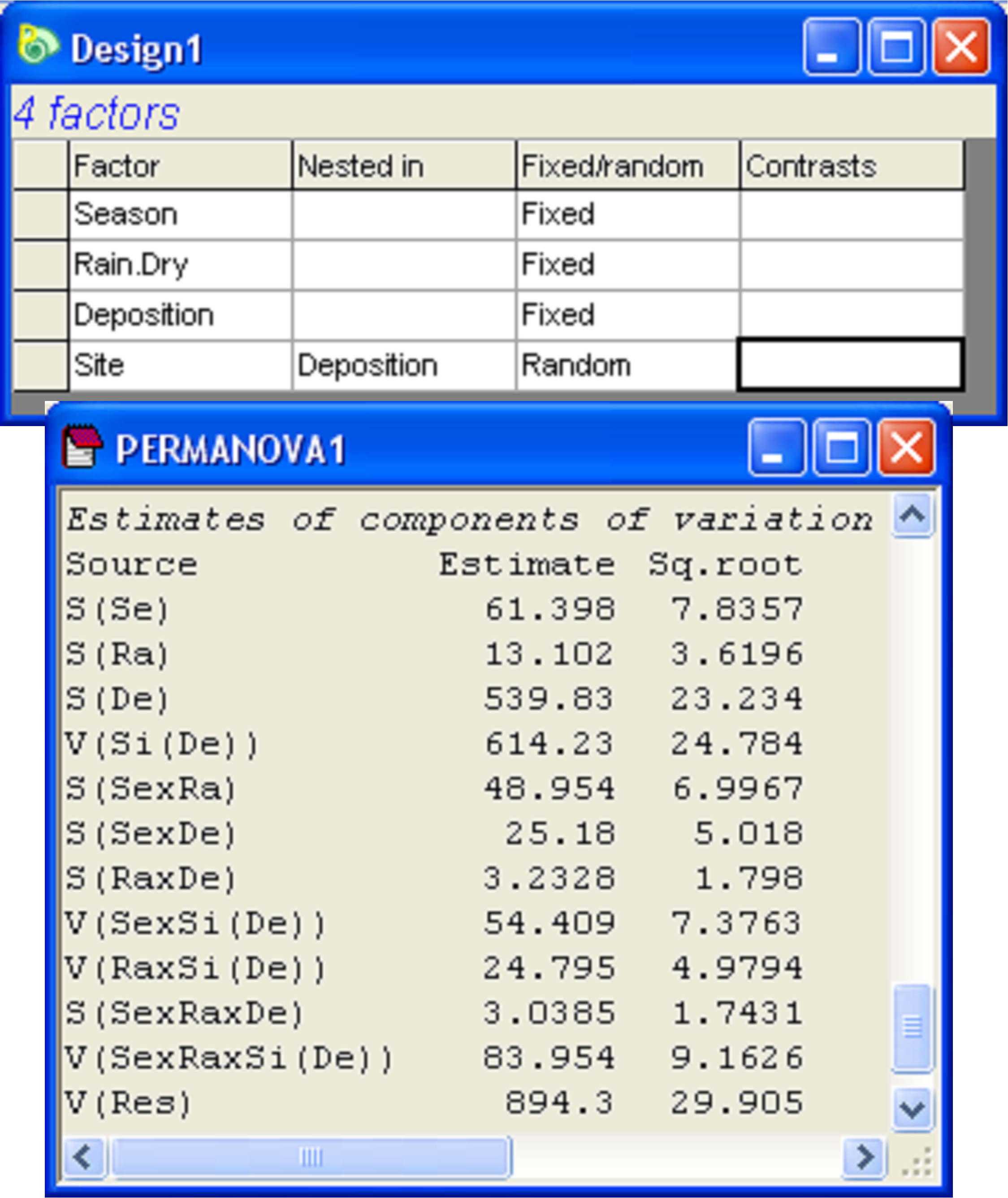
Fig. 3.11. Design file and estimated components of variation from the ensuing PERMANOVA analysis of the Okura macrofaunal data.

A PERMANOVA analysis based on the Bray-Curtis resemblance measure calculated from log(X+1)-transformed variables yielded quantitative measures for the components of variation associated with each term in the model (Fig. 3.11)⁷². Focusing on the main effects for the non-nested factors only, we can see that the greatest effect size was attributable to Deposition, followed by Season, followed by Rain.Dry. To visualise the variation among the relevant cell centroids in this design, we begin by identifying the cells that correspond to what we wish to plot as levels of a single factor. In this case, we wish to examine the cells corresponding to all combinations of Season × Rain.Dry × Deposition. From the full resemblance matrix, choose Edit > Factors > Combine, then click on each of these main effect terms in turn, followed by the right arrow in order to move them over into the ‘Include’ box on the right, then click ‘OK’. Next, to calculate distances among these centroids, choose PERMANOVA+ > Distances among centroids…> Grouping factor: SeasonRain.DryDeposition > OK (Fig. 3.12). The resulting resemblance matrix will contain distances (in Bray-Curtis space, as that is what formed the basis of the analysis here) among the a × b × c = 3 × 2 × 3 = 18 cells. Note that the names of the samples (centroids) in this newly created resemblance matrix will be the same as the levels of the factor that was used to identify the cells. Whereas the original resemblance matrix had 540 samples, we have now obtained Bray-Curtis resemblances among 18 centroids, each calculated as an average (using PCO axes, not the raw data mind!) from d × n = 5 × 6 = 30 cores.

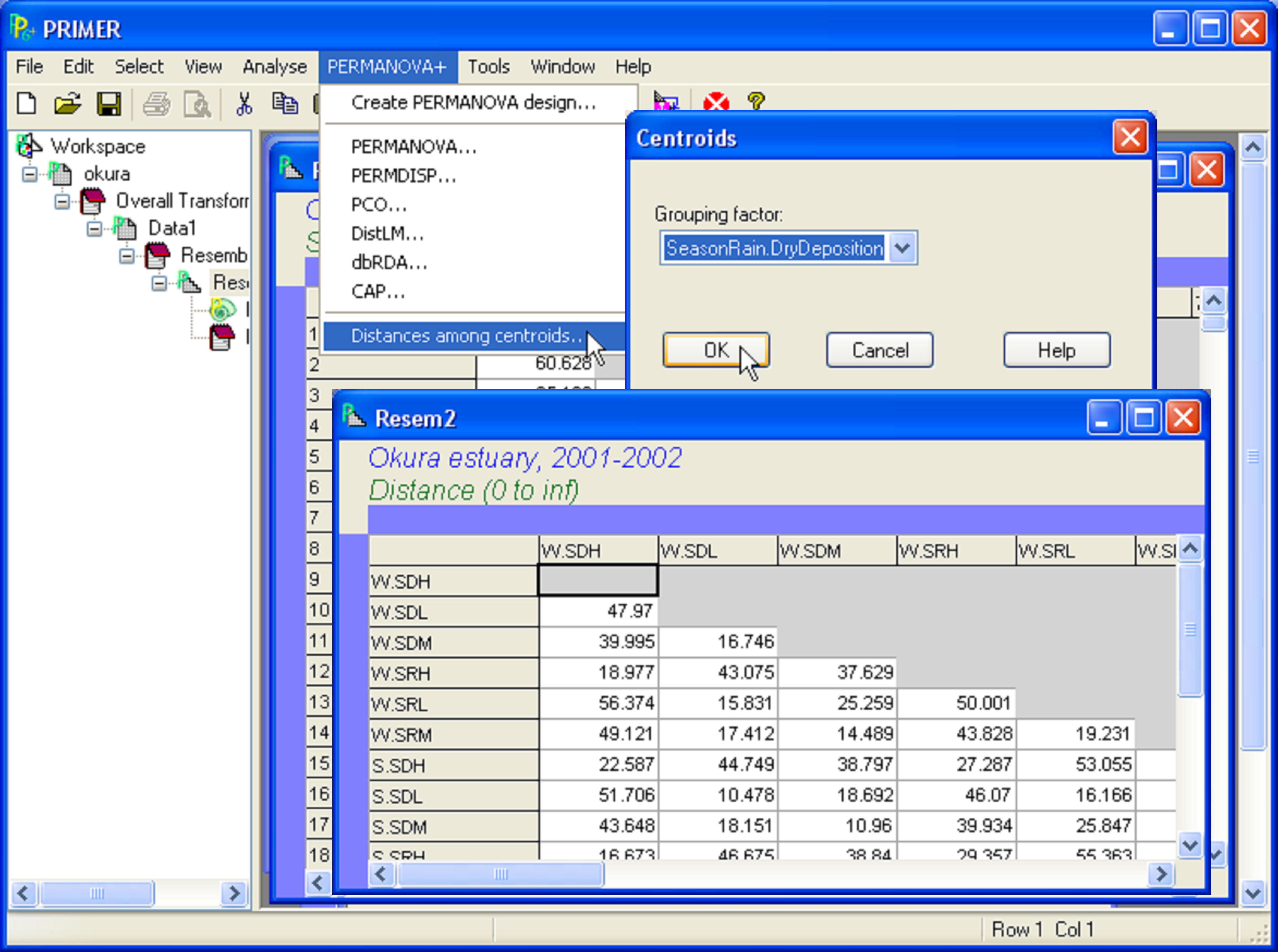Fig. 3.12. Calculating distances among centroids for the Okura data. The centroids are identified by a factor with 18 levels, consisting of all combinations of three factors in the design: ‘Season’, ‘Rain.Dry’ and ‘Deposition’.

From the distance matrix among centroids (‘Resem2’), choose PERMANOVA+ > PCO and examine the resulting ordination of centroids (Fig. 3.13). The first PCO axis explains the majority of the variation among these cells (nearly 75%) and is strongly associated with the separation of assemblages in high depositional environments (on the right) from those in low or medium depositional environments (on the left). Of far less importance (as was also shown in the PERMANOVA output) is the seasonal factor. Differences among seasons are discernible along PCO axis 2, explaining less than 8% of the variation among cells and with an apparent progression of change in assemblage structure from winter/spring, through spring/summer and then to late summer from the top to the bottom of the PCO plot (Fig. 3.13). Of even less importance is the effect of rainfall – the centroids corresponding to the two sampling times within each season and depositional environment occur quite close together on the plot, further indicating that, for these data (and based on the Bray-Curtis measure), seasonal and depositional effects were of greater importance than rainfall effects, which were negligible.

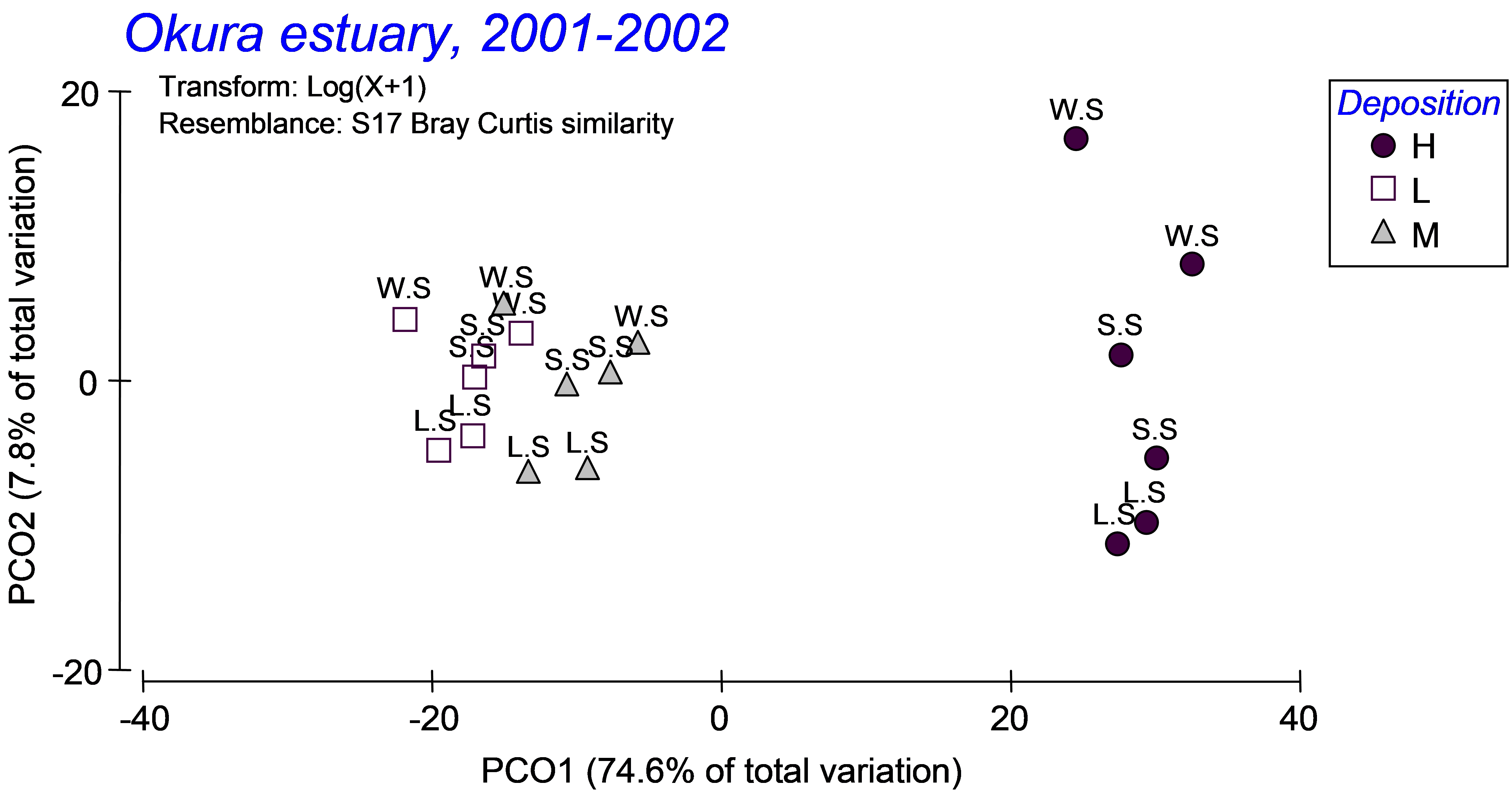
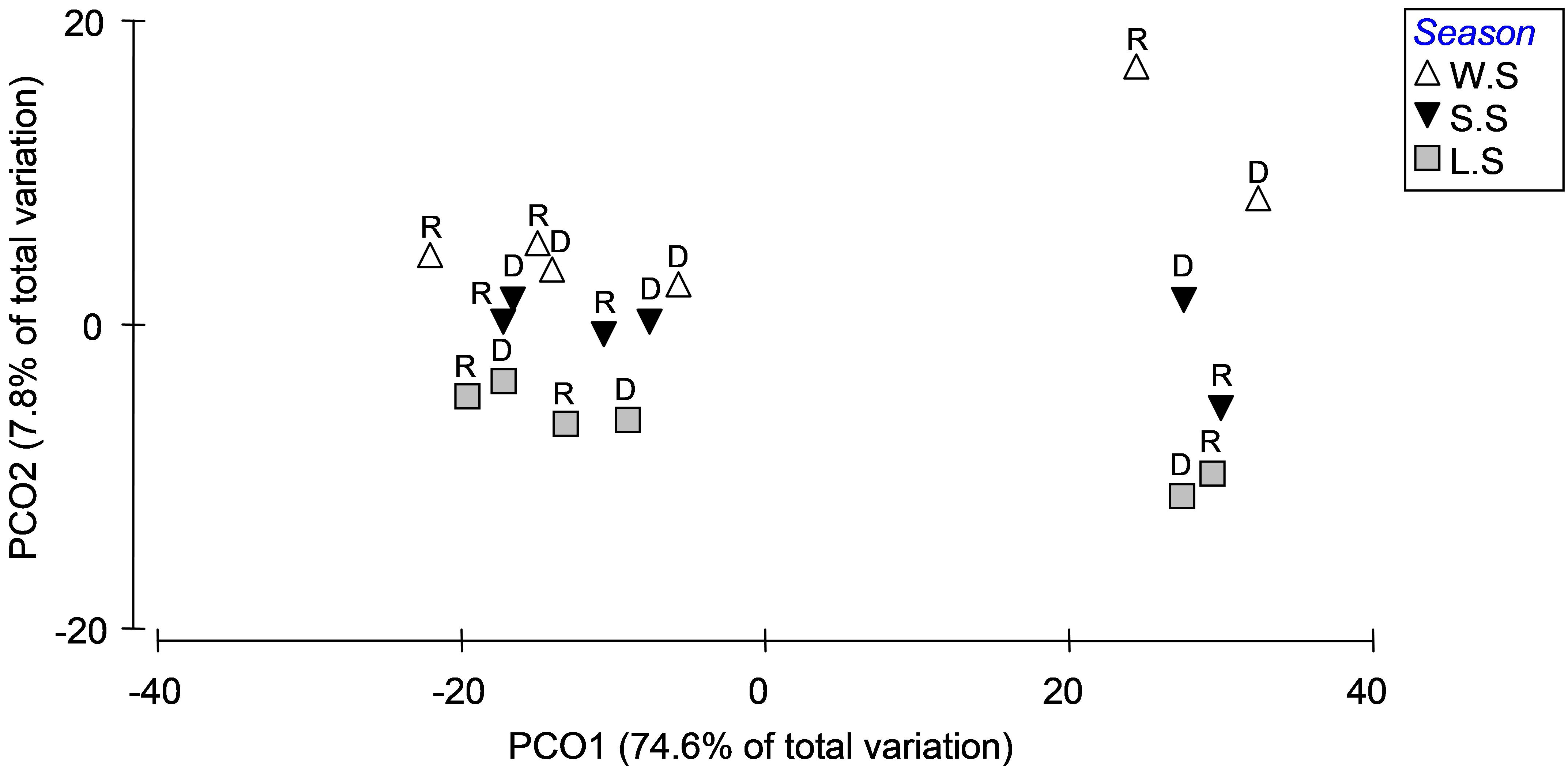Fig. 3.13. PCO of distances among centroids on the basis of the Bray-Curtis measure of log(X+1)-transformed abundances for Okura macrofauna, first with ‘Deposition’ symbols and ‘Season’ labels (top panel) and then with ‘Season’ symbols and ‘Rain.Dry’ labels (bottom panel).

Interactions among these factors did not contribute large amounts of variation, but they were present and some were statistically significant (see the PERMANOVA output in Fig. 3.11). The seasonal effects appeared to be stronger for the high depositional environments than for either of the medium or low depositional environments, according to the plot, so it is not surprising that the Season×Deposition term is sizable in the PERMANOVA output as well. Similarly, the Season×Rainfall interaction term contributes a reasonable amount to the overall variation, and the plot of centroids suggests that rainfall effects (i.e. the distances between R and D) were more substantial in winter/spring than in late/summer. Of course, ordination plots of appropriate subsets of the data and relevant pair-wise comparisons can be used to further elucidate and interpret significant interactions.

This example demonstrates that ordination plots of distances among centroids can be very useful in unraveling patterns among levels of factors in complex designs. The new tool Distances among centroids in PERMANOVA+ uses PCO axes to calculate these centroids, retaining the necessary distinctions between sets of axes that correspond to positive and negative eigenvalues, respectively, and so maintaining the multivariate structure identified by the choice of resemblance measure as the basis for the analysis as a whole.

Importantly, an analysis that proceeds instead by first calculating centroids (averages) from the raw data first, followed by the rest (i.e. calculating the transformation and Bray-Curtis resemblances on these averages) would not provide the same results. Patterns from the latter would also not necessarily accord with the relative sizes of components of variation from a PERMANOVA partitioning that had been performed on the full set of data. We recommend that the decision to either sum or average the raw data before analysis should be driven by an a priori judgment regarding the appropriate scale of observation of the communities of interest. For example, in some cases, the individual replicates are too small and too highly variable in composition to be considered representative samples of the communities of interest. In such cases, pooling together (summing or averaging) small-scale replicates to obtain an appropriate sample unit for a given spatial scale before performing a PERMANOVA (or other) analysis may indeed be appropriate⁷³. The tool provided here to calculate distances among centroids, instead, assists in understanding the partitioning of the variation in the multivariate space identified by the resemblance measure, well after a decision regarding what should comprise an appropriate lowest-level representative sampling unit has been made.

---

⁷² See chapter 1 for a more complete description of how to use the PERMANOVA routine to analyse complex experimental designs.

⁷³ An example where this was done was the Norwegian macrofauna (norbio.pri in the ‘NorMac’ folder), where 5 benthic grabs at a site were pooled together and considered as a single sampling unit for analysis.