1.29 Pooling or excluding terms

For a given design file, PERMANOVA, by default, will do a partitioning according to all terms that are directly implied by the experimental design. For multi-factor designs, PERMANOVA will assume that all factors are crossed with one another, unless nesting is specified explicitly in column 2 of the design file. Although a factor cannot interact with a factor within which it is nested, factors that are crossed with one another necessarily generate interaction terms, and this full model (having all possible interactions) is generated by default.

In some cases, however, one may wish to remove one or more terms from a given model. There are various reasons for wishing to remove individual terms, including:

  (i) lack of evidence against the null hypothesis of that term’s component being equal to zero;
  (ii) a negative estimate of that term’s component of variation;
  (iii) previous studies have determined that term’s component to be zero or negligible;
  (iv) hypotheses of interest require tests of models that exclude one or more particular terms.

The user should be aware, however, that removing a term from a model equates with the assertion that its component of variation (that is, either S(*) or V(*) for a fixed or a random term, respectively, as the case may be) is equal to zero. By asserting that a component is equal to zero, one effectively combines, or pools, that term’s contribution (and its associated degrees of freedom) with some other term in the model. In the dialog of the PERMANOVA routine, we make a distinction between two different ways of removing a term:

• Excluding a term from the model – in which case the term is completely excluded and is not considered as ever having been part of the model in any form. Regardless of where the term occurs in the structure of the experimental design, excluding a term in this way is equivalent to pooling the df and SS for that term with the residual df and SS;
• Pooling a term – in which case the df and SS for that term is pooled with the term (or terms) which have equivalent EMS’s after that term’s component of variation is set to zero. For example, in a fully hierarchical design, this would correspond to a term being pooled with the term occurring immediately below it within the structure of the design.

Complete exclusion of a term might be done, for example, in cases where we wish to construct a particular model that fully ignores those terms (e.g., in designs that lack replication, see the section on Split-plot designs below). This is done by clicking on the ‘Terms…’ button in the PERMANOVA dialog. More generally, however, the removal of terms should be done with correct and appropriate pooling, where the component of variation for that term is set to zero and the EMS’s for the other terms in the model are re-evaluated. Pooling like this should be done, for example, to sequentially remove terms from a model having negative estimates for components of variation (e.g., Fletcher & Underwood (2002) ), or to remove terms having large P-values. In PERMANOVA, this is done by clicking on the ‘Pool…’ button in the PERMANOVA dialog.

With respect to pooling on the basis of the reason given in (i) above, the assertion that a given term’s component is equal to zero should be made with some caution. Although a P-value > 0.05 (under the usual scientific convention) may not provide sufficient evidence to reject the null hypothesis (H$_0$), failing to reject H$_0$ is nevertheless logically very different from asserting that H$_0$ is true ( Popper (1959) , Popper (1963) )! There are differences of opinion regarding how large the P-value for a given term should be before the assertion of H$_0$ to remove that term might be justified (e.g., Hines (1996) , Janky (2000) ). “To pool or not to pool” is a decision left to the user, but we note that many practicing scientists use the rule-of-thumb suggested by Winer, Brown & Michels (1991) and Underwood (1997) that the P-value should exceed 0.25 before removing (i.e. pooling) any given term.

Pooling a single term has important consequences for the construction of pseudo-F ratios, P-values and the estimation of components for the remaining terms. Thus, it is generally unwise to remove more than one term at a time (unless there are sufficient a priori reasons for doing so). The general rule suggested by Thompson & Moore (1963) and Fletcher & Underwood (2002) is, when faced with more than one term which might be removed from a given model, remove only one term at a time, beginning with the term having the smallest mean square, and at each step re-assess whether more terms should be removed or not.

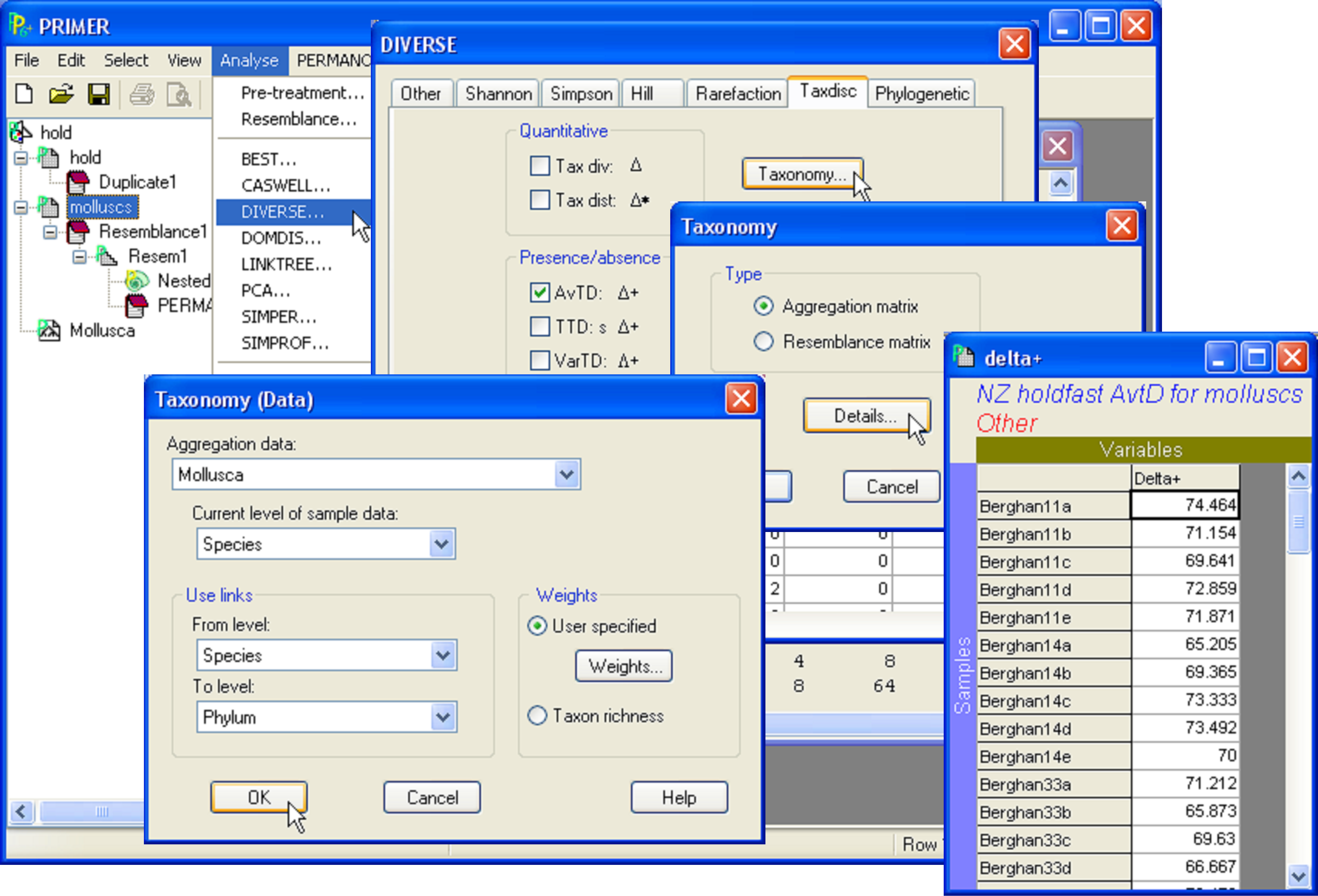Fig. 1.30. Calculating the average taxonomic distinctness of molluscs for New Zealand holdfast assemblages.

As an example of pooling, consider the New Zealand holdfast assemblages discussed in the previous two sections. Here, we shall focus on the analysis of a single variable – the average taxonomic distinctness (AvTD, $\Delta +$, Warwick & Clarke (1995) ) for molluscs in holdfasts. Open up the file hold.pwk and, from within this workspace, open up the aggregation file for the molluscs, called Mollusca.agg. Next, highlight the molluscs worksheet (see the section Nested design above for details on obtaining this worksheet). Use the built-in tool in PRIMER to obtain the average taxonomic distinctness in each sample as a worksheet: select Analyse > Diverse and remove the $\checkmark$ in front of all of the default options except for ($\checkmark$AvTD: $\Delta +$) shown under the ‘Taxdisc’ tab & ($\checkmark$Results to worksheet) (Fig. 1.30). (Note that this also requires clicking on each of the ‘Other’, ‘Shannon’ and ‘Simpson’ tabs, in turn, in order to remove the $\checkmark$ for those options as well). Rename the resulting worksheet delta+ (which should contain only one variable, ‘Delta+’) and select Edit > Properties to give it the title: NZ holdfast AvTD for molluscs.

Next, from the delta+ worksheet, calculate a Euclidean distance resemblance matrix: Analyse > Resemblance > (Analyse between •Samples) & (Measure •Euclidean distance). Do the analysis on the basis of the nested design (see the design file in Fig. 1.29) using the PERMANOVA routine with (Design worksheet: Nested design) & (Num. permutations: 9999) and all other choices as per the defaults. This analysis will result in an ANOVA partitioning (yielding values for df, SS, MS, F ratios and estimates of variance components) equivalent to that obtained using classical univariate ANOVA. (The data in this worksheet can be exported and analysed using a different statistical package to confirm this). The only difference will lie in the P-values, which of course are obtained using permutations in PERMANOVA, as opposed to using the traditional tables of the F distribution which rely on the assumption of normality.

The results suggest that there is no significant variability in AvTD for molluscs among different sites (Fig. 1.31). Furthermore, the P-value for ‘Si(Lo)’ is quite large (P > 0.90) and the estimate of the variance component for ‘Si(Lo)’ is negative. Thus, using the rationale of either (i) or (ii) above, we may remove this term from the model by pooling it.

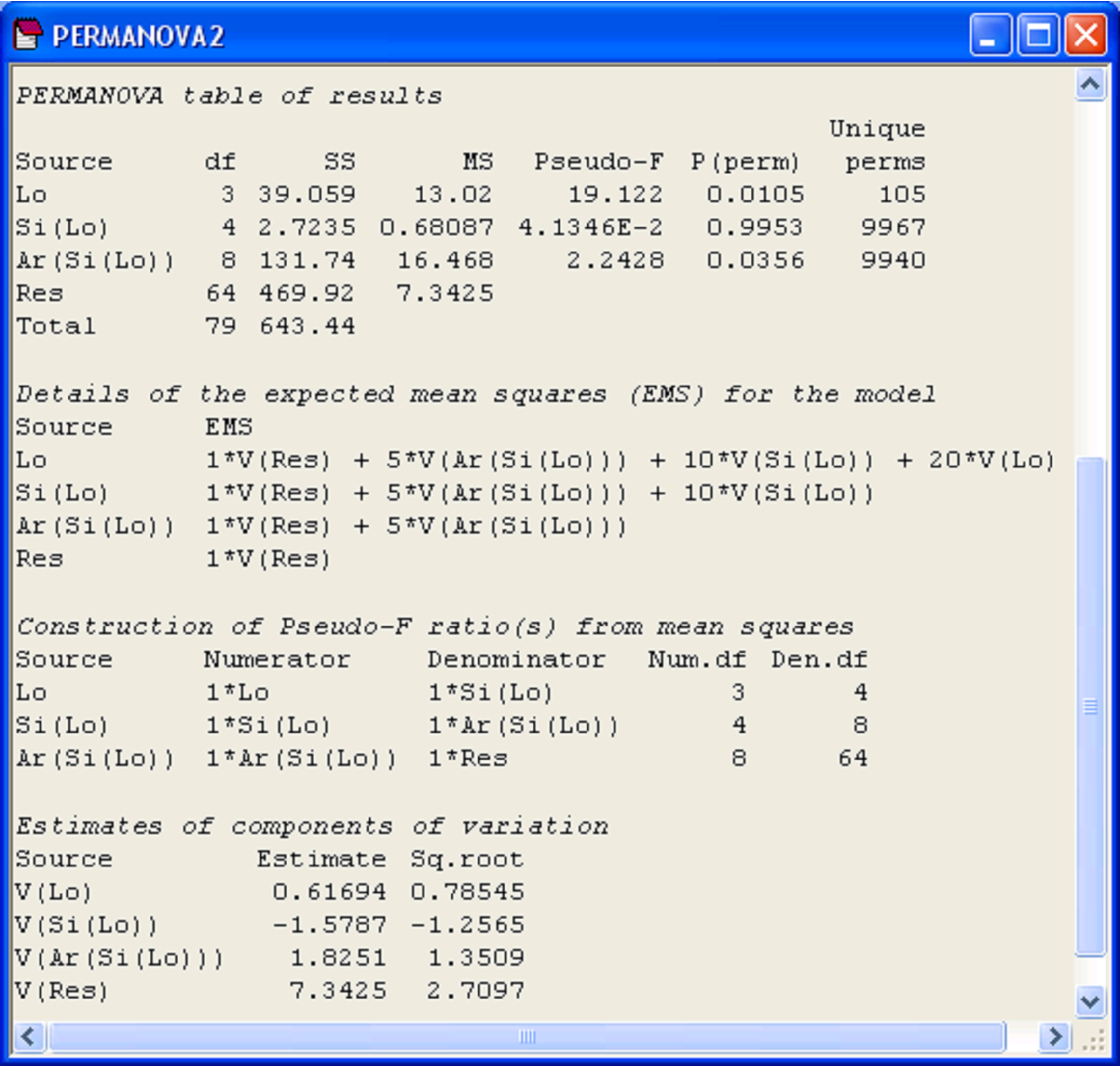Fig. 1.31. Results of PERMANOVA for the full 3-factor nested model on AvTD of molluscs.

This is achieved relatively easily, by re-running the PERMANOVA routine on the basis of the same design file, but this time, click on the ‘Pool…’ button (Fig. 1.32). A new dialog box appears entitled ‘Selection’ with a list of all of the terms in the model. The user may choose which terms in the model to pool. For the present case, we wish to pool the ‘Si(Lo)’ term. In the ‘Available’ box, click on the term Si(Lo) followed by to move this into the ‘Include’ box, then ‘OK’.

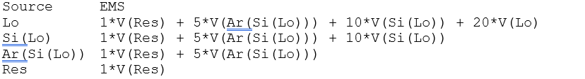
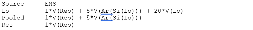
To understand how pooling is done in the PERMANOVA routine, consider the details of the EMS in the present example for the full model before pooling:

By pooling the term ‘Si(Lo)’, we are explicitly asserting that the component V(Si(Lo)) = 0. Setting this component deliberately to zero wherever it appears yields the following:

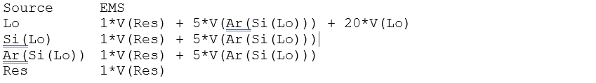
Thus, the mean square for the term ‘Si(Lo)’ and the mean square for the term ‘Ar(Si(Lo))’ are now estimating the same thing, i.e. they have the same expectation. This means that their SS and df can be added together to obtain a pooled MS, as follows:

$$ MS _ {pooled} = \frac {\left( SS _ {Si(Lo)} + SS _ {Ar(Si(Lo))} \right) } { \left( df _ {Si(Lo)} + df _ {Ar(Si(Lo))} \right) } \tag{1.5} $$

The PERMANOVA output file from the analysis after pooling identifies which terms were pooled, under the heading ‘Pooled terms’ and also identifies the terms whose SS and df were combined as a consequence of this (Fig. 1.32). The new pooled term is given a unique name – it is simply called ‘Pooled’ in the present case. In the event of there being more terms to pool, potentially more than one pool of terms may occur in a single analysis. This is also catered for by the PERMANOVA routine, if required, with each pool identified by its component terms and given its own unique name. The EMS’s after pooling in the present case are:

and the associated degrees of freedom for the pooled term are:

$$ df _ {Pooled} = \left( df _ {Si(Lo)} + df _ {Ar(Si(Lo))} \right) = \left( 4 + 8 \right) = 12 \tag{1.6} $$

Pooling the ‘Si(Lo)’ term has resulted in all of the remaining estimated components of variation in the model being non-negative. It has also, however, substantially changed the F-ratios and tests for the remaining terms. The term ‘Lo’ is now not statistically significant (pseudo-F = 1.16, P = 0.36, Fig. 1.32), whereas before, when tested using the mean square for ‘Si(Lo)’ as the denominator, it was (pseudo-F = 19.1, P = 0.01, Fig. 1.31). This is an important point. Although pooling may result in an increase in power, caused by an increase in the denominator df for the test of a given term (here, ‘Den.df’ for the test of ‘Lo’ has gone up from 4 to 12), this is also often off-set by an increase in the denominator MS for the test after pooling (cf. $MS _ {Si(Lo)} = 0.68$, whereas $MS _{Pooled} = 11.2$), which reduces the value of pseudo-F for the test. It is usually not possible to tell a priori just how the tests for other terms in the model will be affected by pooling. Clearly, however, estimated components of variation, pseudo-F ratios and P-values will be affected by pooling. Thus, as stated previously, pooling should only be done one term at a time. From the present analysis, after pooling, there is apparently no statistically significant variability in the AvTD of molluscs among holdfasts at any of the spatial scales examined (Locations, Sites or Areas).

Note that these results (Fig. 1.32), obtained by removing the ‘Si(Lo)’ term using the ‘Pool…’ button in the PERMANOVA dialog, are not the same as the results that would have been obtained if we had simply excluded ‘Si(Lo)’ from the model entirely, using the ‘Terms…’ button. In that case, the term would have been considered to be non-existent. It would not have been included in the partitioning at all and its SS and df would therefore have ended up as part of the residual. This is clearly illogical and undesirable in the present case. Removing the ‘Si(Lo)’ term should result in an increase to the df associated with the denominator MS being used to test the ‘Lo’ term (i.e., its SS and df should be combined with the ‘Ar(Si(Lo))’ term), and not merely ignored and added to the residual variation. Another possibility would be to re-cast the model with two factors: ‘Lo’ and ‘Ar(Lo)’, but we would need to be careful and make sure that the areas within any location (even those from different sites) each had a unique name in the specification of the ‘Areas’ factor levels.

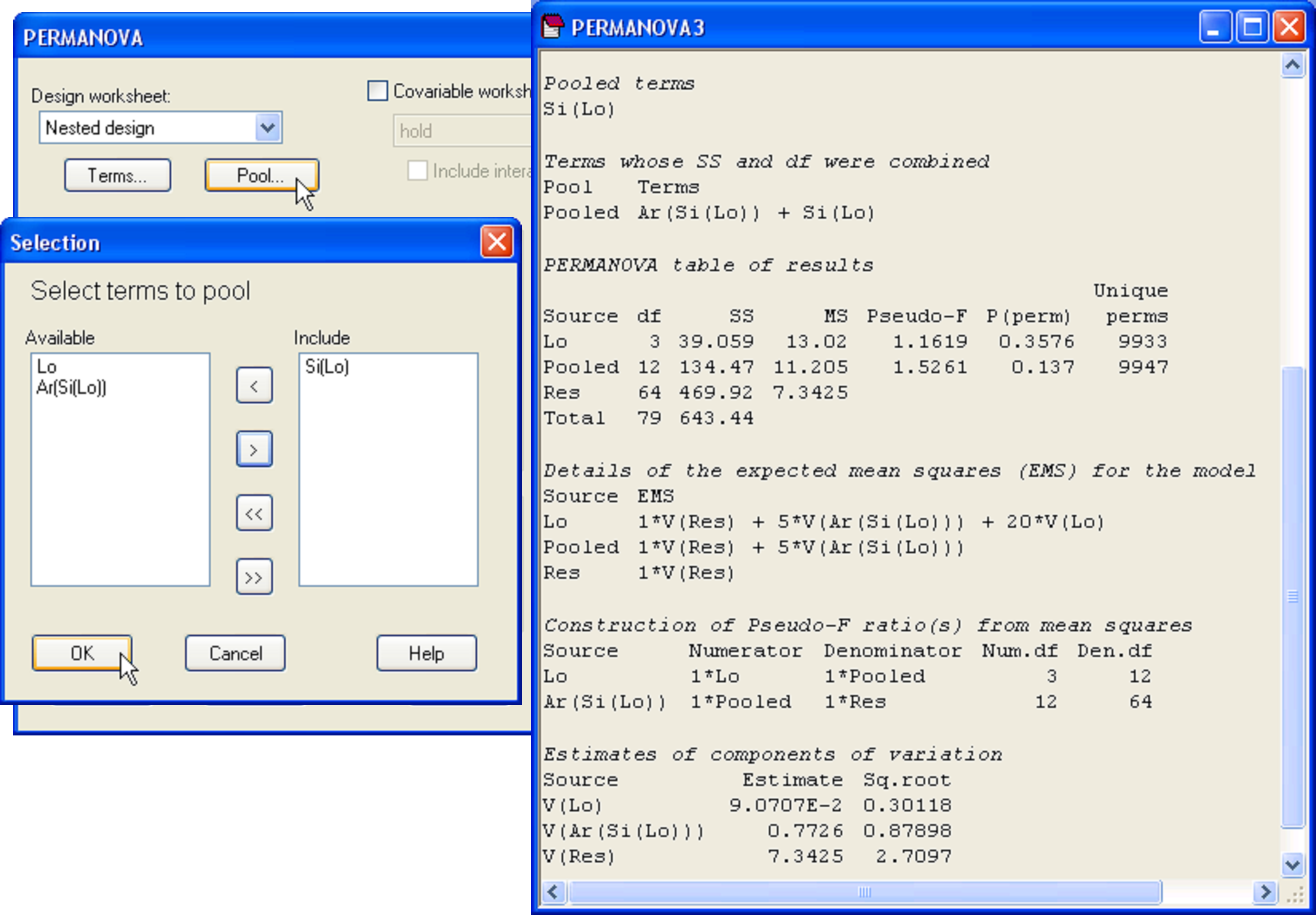
Fig. 1.32. Dialog to pool the ‘Si(Lo)’ term and results for the PERMANOVA analysis of the AvTD of molluscs after pooling.

If pooling of a given term would result in its being combined with the residual in any event (which of course, occurs legitimately in some cases), then the results using these two approaches will be equivalent. Otherwise, however, they will not. We consider that removal of terms using the ‘Pool…’ button will be most appropriate for the majority of situations. The use of the ‘Terms…’ button to exclude terms entirely may be useful, however, to craft specific simplified models in the event that replication is lacking (see the section Designs that lack replication). The dialog available under the ‘Terms…’ button can also be used to change the order in which individual terms are fitted. Although the order in which terms are fitted is of no consequence for balanced ANOVA designs, it is important for analyses of unbalanced designs or designs including covariates using Type I (sequential) SS (see the sections Unbalanced designs and Designs with covariates).