2.12 Dispersion in crossed designs (Cryptic fish)
When two factors are crossed with one another, there may be several possible hypotheses concerning relative dispersions among groups. An important aspect of analysing multi-factorial designs is to keep straight when you are focusing on dispersion effects and when you are focusing on location effects. Running PERMANOVA and PERMDISP in tandem, driven by carefully articulated hypotheses, provides a useful general approach.
Here we shall consider a study to investigate effects of marine reserve status and habitat on cryptic fish assemblages in northeast New Zealand, as described by Willis & Anderson (2003) . Although marine reserves in this region afford protection for larger exploited fish species (such as snapper, Pagrus auratus, which occur in greater relative abundances and sizes inside reserves, see Willis, Millar & Babcock (2003) ), relatively little is known regarding the potential flow-on effects (either positive or negative) on many of the other components of these ecosystems (but do see Shears & Babcock (2002) , Shears & Babcock (2003) regarding habitat-scale effects). For example, do assemblages of smaller and/or more cryptic fish (such as triplefins and gobies) change with increased densities of predators inside versus outside marine reserves? Is this effect (if any) modified in kelp forest habitat as opposed to urchin-grazed ‘barrens’ habitat? The two factors in the design were:
-
Factor A: Status (fixed with a = 2 levels, reserve (R) or non-reserve (N) sites).
-
Factor B: Habitat (fixed with b = 2 levels, kelp forest (k) or urchin-grazed rock flats (r), crossed with Status).
There were n = 6 replicate 9 m$^2$ plots surveyed within each of the a × b = 4 combinations of levels of the above two factors, yielding counts of abundances for p = 33 species. These data are located in the file cryptic.pri in the ‘Cryptic’ folder of the ‘Examples add-on’ directory. An MDS on the basis of the Bray-Curtis measure on square-root transformed abundances does not show very clear effects of either of these factors (Fig. 2.15). Formal tests are necessary to clarify whether any significant effects of either factor (or their interaction) are detectable in the higher-dimensional multivariate space.
 Fig. 2.15. MDS of cryptic fish assemblages at reserve (R) or non-reserve (N) sites in either kelp forest or urchin-grazed rock flat habitats.
First, we shall run a PERMANOVA on the two-factor design, bearing in mind that the test is specifically designed to detect location effects, but dispersion effects (if any) might also be detected by this test. Results indicate that the two factors do not interact (P > 0.70), but there are significant independent effects of ‘Status’ and ‘Habitat’ (P < 0.01 in each case, Fig. 2.16).
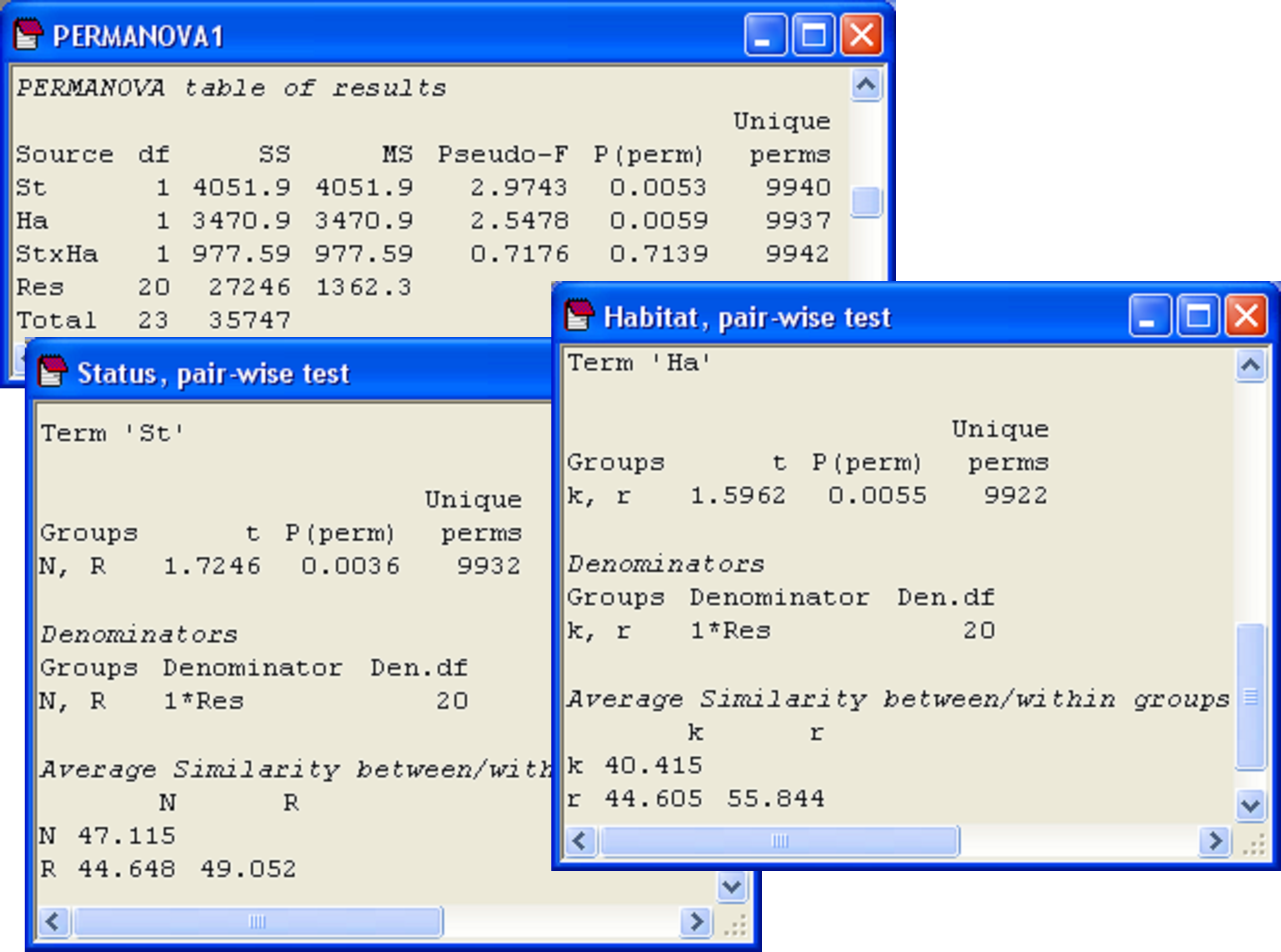 Fig. 2.16. PERMANOVA for the two-way analysis of cryptic fish, along with pair-wise comparisons for each of the main effects.
Although there are only two levels of each of the factors (so the tests in the main PERMANOVA analysis are enough to indicate the significant difference between the two levels, in each case), pair-wise comparisons done on each factor will give us a little more information regarding the average similarity between and within the different groups (Fig. 2.16). The average within-group similarities are comparable for ‘N’ and ‘R’, but the average within-group similarity in the kelp forest habitat (‘k’, 40.4%) is much smaller than that in the rock flat habitat (‘r’, 55.8%). The former is even smaller than the average similarity between kelp and rock-flat habitats (44.6%)! The pattern in the MDS plot (Fig. 2.15) also indicates greater dispersion of points for ‘k’ (squares) than for ‘r’ (downward triangles). These observations provide signals to suggest (but do not prove) that the significant effect of habitat might be driven somewhat by differences in dispersions. Of course, we can investigate this idea formally using PERMDISP.
First, although there is no significant interaction detected by PERMANOVA, it is still possible that the individual cells may differ in their relative dispersions. This can be tested by combining the two factors to make a single factor with a × b = 4 levels and then running PERMDISP to compare these within-cell dispersions. Choose Edit > Factors > Combine and then ‘Include’ both factors in the ‘Ordered selection’ dialog box (Fig. 2.17). Next choose PERMANOVA+ > PERMDISP > (Group factor: StatusHabitat) & (Distances are to •Centroids) & (P-values are from •Permutation) & (Num. permutations: 9999). For these data, the null hypothesis of equal dispersions among the four cells is retained (F = 2.0, P > 0.25, Fig. 2.17).
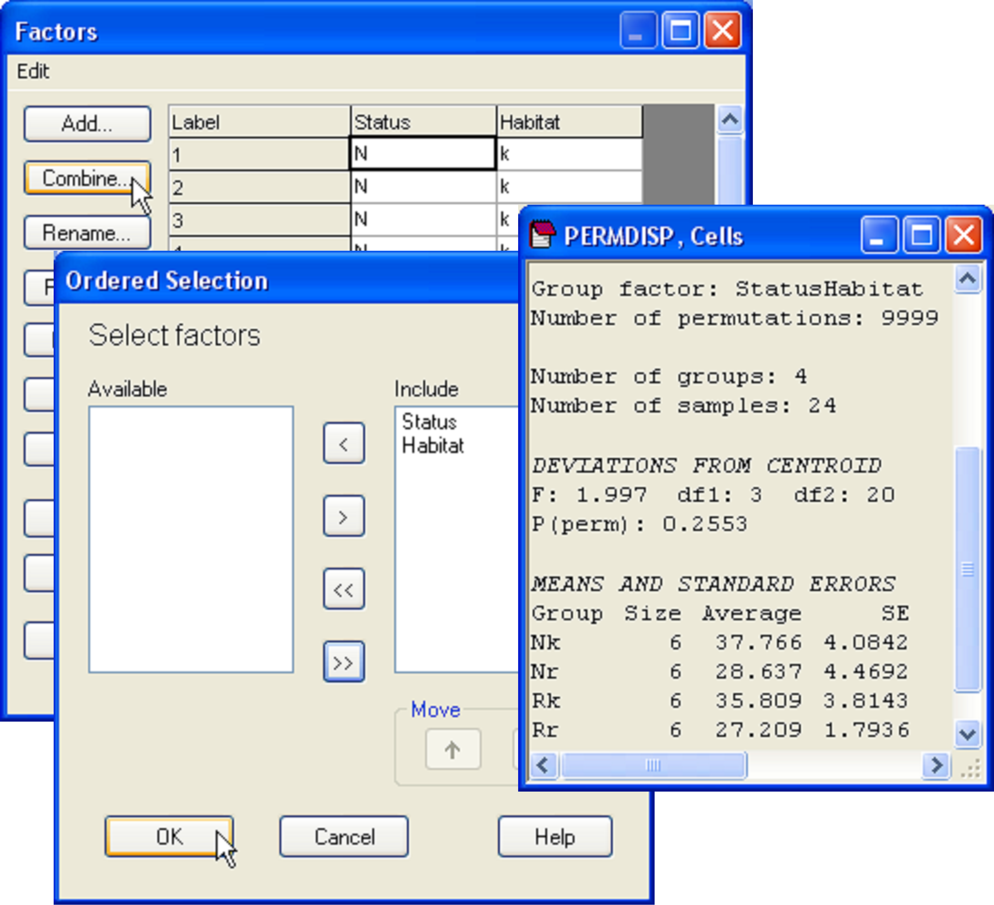 Fig. 2.17.
Menus used to generate a combined factor consisting of the 4 combinations of ‘Status’ and ‘Habitat’, and the results window from PERMDISP which formally compares dispersions among these four cells.
Fig. 2.17.
Menus used to generate a combined factor consisting of the 4 combinations of ‘Status’ and ‘Habitat’, and the results window from PERMDISP which formally compares dispersions among these four cells.
Next, to consider analyses of dispersions for main effects in a crossed design (such as this), it is important to consider what might be meaningful in light of the PERMANOVA results. When two (or more) factors are crossed with one another, it is easily possible to confuse a dispersion effect with an interaction effect. To illustrate this point, suppose I have a two-factor design, where there is a significant interaction such as that shown in Fig. 2.18. More specifically, suppose there is no effect of factor A in level 1 of factor B (grey/filled symbols), but there is a significant effect of factor A in level 2 of factor B (white/open symbols). A test for equality of dispersions among the levels of factor B that ignored A would clearly find a significant difference between the two levels of factor B (with white symbols obviously being more dispersed than grey symbols). However, this is not really caused by dispersion differences per se, but rather is due to the fact that factor A interacts with factor B. Therefore, before performing tests of dispersion for main effects in crossed designs, the potential for interactions to confound interpretations of the results should be examined. This is generally achieved by first testing and investigating the nature of any significant interaction terms using PERMANOVA, and also by examining patterns in ordination plots.
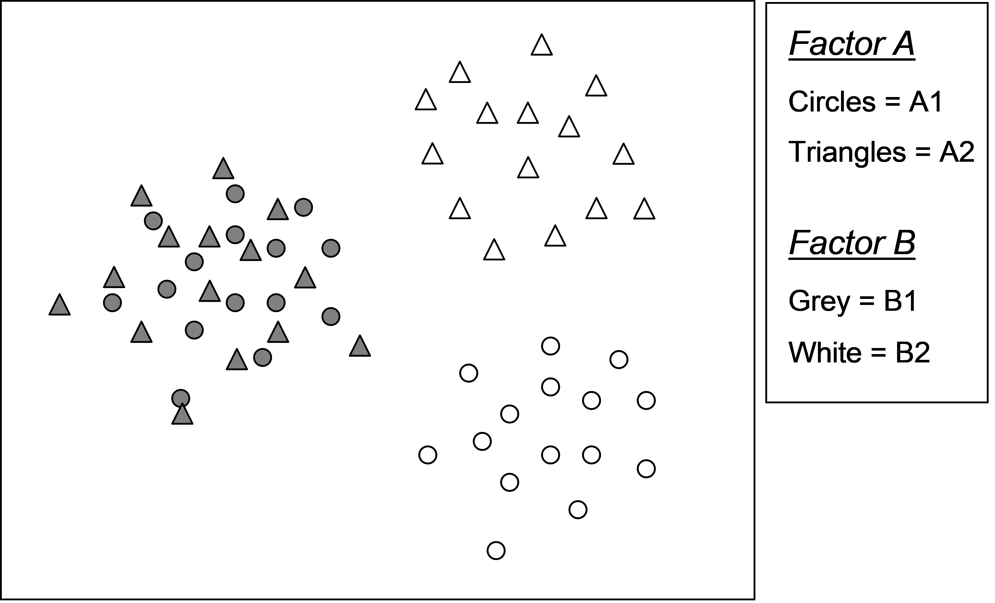
Fig. 2.18. Schematic diagram in two dimensions of an interaction between two factors that can result in misinterpretation of tests of dispersion for main effects.
We have seen, for the cryptic fish data, that no interaction was detected between ‘Status’ and ‘Habitat’ (Fig. 2.16), so we can perform the test of homogeneity of dispersions for each of the main effects separately (ignoring the other factor) using PERMDISP. These reveal no significant differences in dispersion for the ‘Status’ factor (F = 0.06, P > 0.82), but significant differences in dispersion for the ‘Habitat’ factor, with greater variability in the fish assemblages observed in kelp forests compared to the urchin-barrens rock flat habitat (F = 7.8, P < 0.05, Fig. 2.19)60.
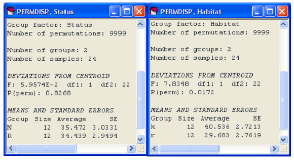
Fig. 2.19. Results of PERMDISP on each of the main effects from the two-factor study of cryptic fish.
Note that the significant effect of the marine reserve ‘Status’ detected by the PERMANOVA is therefore now interpretable to be purely (in essence) a location effect, as the test for homogeneity of dispersions for this factor was not significant. However, the effect of ‘Habitat’ appears to be primarily (although perhaps not entirely) driven by differences in dispersion, with greater variability in the structure of cryptic fish assemblages observed in kelp forest habitats compared to rock flat habitats. If there is a location effect (i.e. a shift in multivariate space) due to habitat in addition to the dispersion effect detected (which of course is possible), then this should be discernible in MDS plots (preferably carried out separately for each reserve status in 3-d, when the stress will drop to lower values than in Fig. 2.15).
60 A word of warning: PERMDISP analyses and measures of dispersion for main effects like this will include the location shifts (if any) of other main effects. Although this won’t necessarily confound the analysis if the factors do not interact, it can nevertheless compromise power. Ideally, we would like to remove location effects of all potential factors before proceeding with the test. This is not implemented in the current version of PERMDISP, but there is clearly scope for further development here.