1.6 Test by permutation

An appropriate distribution for the pseudo-F statistic under a true null hypothesis is obtained by using a permutation (or randomization) procedure (e.g., Edgington (1995) , Manly (2006) ). The idea of a permutation test is this: if there is no effect of the factor, then it is equally likely that any of the individual factor labels could have been associated with any one of the samples. The null hypothesis suggests that we could have obtained the samples in any order by reference to the groups, if groups do not differ. So, another possible value of the test statistic under a true null hypothesis can be obtained by randomly shuffling the group labels onto different sample units. The random shuffling of labels is repeated a large number of times, and each time, a new value of pseudo-F, which we will call pseudo-$F ^ \pi$, is calculated (Fig. 1.5). Note that the samples themselves have not changed their positions in the multivariate space at all as a consequence of this procedure, it is only that the particular labels associated with each sample have been randomly re-allocated to them (Fig. 1.5).

If the null hypothesis were true, then the pseudo-F statistic actually obtained with the real ordering of the data relative to the groups will be similar to the values obtained under permutation. If, however, there is a group effect, then the value of pseudo-F obtained with the real ordering will appear large relative to the distribution of values obtained under permutation.

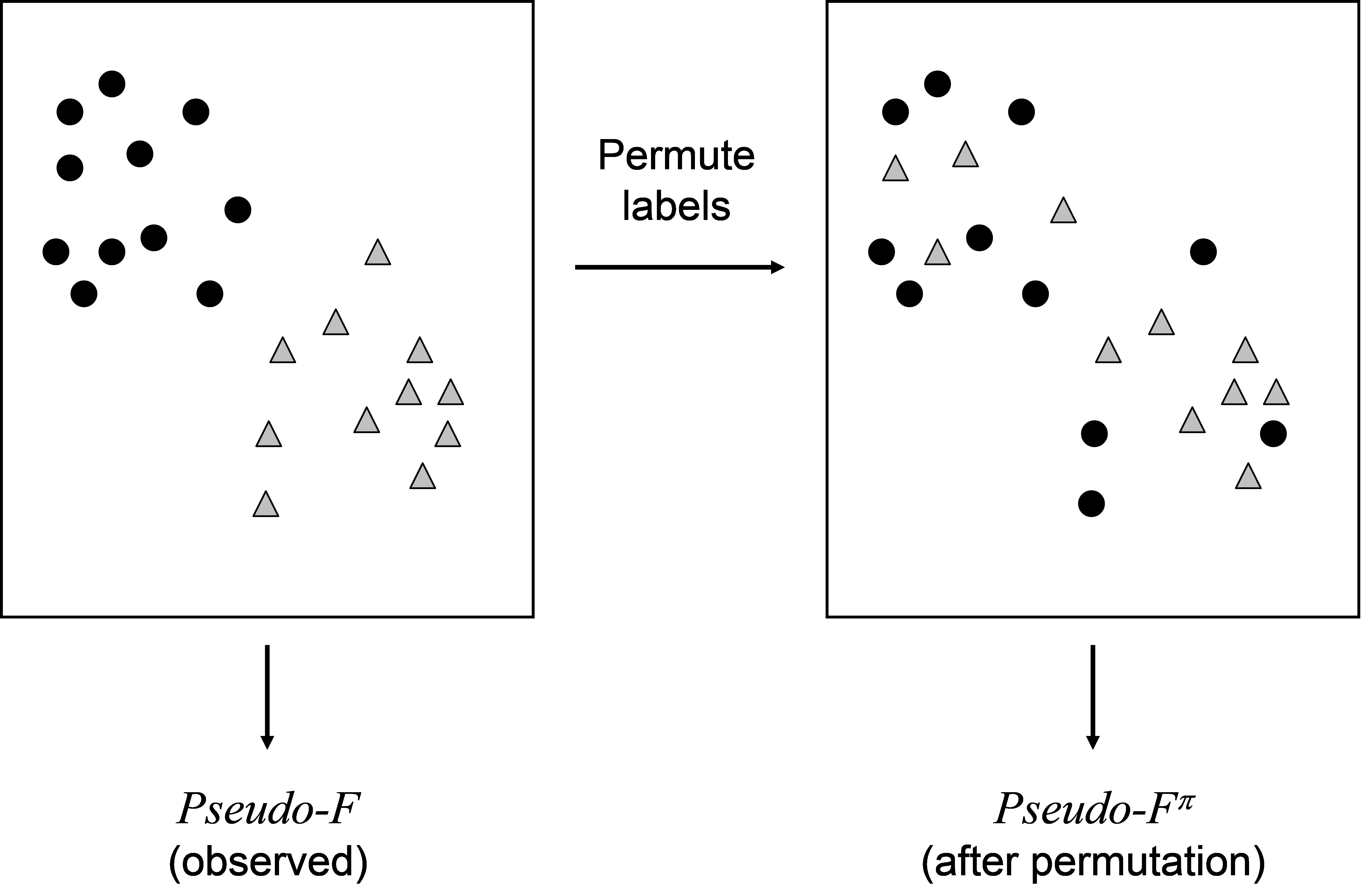Fig. 1.5. After calculating an observed value of the test statistic, a value that might have been obtained under a true null hypothesis is calculated by permuting labels.

The frequency distribution of the values of pseudo-$F ^ \pi$ is discrete: that is, the number of possible ways that the data could have been re-ordered is finite. The probability associated with the test statistic under a true null hypothesis is calculated as the proportion of the pseudo-$F ^ \pi$ values that are greater than or equal to the value of pseudo-F observed for the real data. Hence,

$$ P = \frac{ \left( \text{No. of } F ^ \pi \ge F \right) +1}{ \left( \text{Total no. of } F ^ \pi \right) +1} \tag{1.4} $$

In this calculation, we include the observed value as a member of the distribution, appearing simply as “+1” in both the numerator and denominator of (1.4). This is because one of the possible random orderings of the data is the ordering we actually got and its inclusion makes the P-value err slightly on the conservative side ( Hope (1968) ) as is desirable.

For multivariate data, the samples (either as whole rows or whole columns) of the data matrix (raw data) are simply permuted randomly among the groups. Note that permutation of the raw data for multivariate analysis does not mean that values in the data matrix are shuffled just anywhere. A whole sample (e.g., an entire row or column) is permuted as a unit; the exchangeable units are the labels associated with the sample vectors of the data matrix (e.g., Anderson (2001b) )¹¹. For the one-way test, enumeration of all possible permutations (re-orderings of the samples) gives a P-value that yields an exact test of the null hypothesis. An exact test is one where the probability of rejecting a true null hypothesis is exactly equal to the a priori chosen significance level ($\alpha$). Thus, if $\alpha$ were chosen to be 0.05, then the chance of a type I error for an exact test is indeed 5%.

In practice, the possible number of permutations is very large in most cases. A practical strategy, therefore, is to perform the test using a large random subset of values of pseudo-$F ^ \pi$ , drawn randomly, independently and with equal probability from the distribution of pseudo-$F ^ \pi$ for all possible permutations. PERMANOVA does not systematically do all permutations, but rather draws a random subset of them, with the number to be done being chosen by the user. Such a test is still exact ( Dwass (1957) ). However, separate runs will therefore result in slightly different P-values for a given test, but these differences will be very small for large numbers of permutations (e.g., in the 3rd decimal place for 9999 permutations) and should not affect interpretation.

Once again, as a rather nice intuitive bonus, PERMANOVA done on one response variable alone and using Euclidean distance yields Fisher’s traditional univariate F statistic. So, PERMANOVA can also be used to do univariate ANOVA but where P-values are obtained by permutation (e.g., Anderson & Millar (2004) ), thus avoiding the assumption of normality. Note also that if the univariate data do happen to conform to the traditional assumptions (normality, etc.), then the permutation P-value converges on the traditional normal-theory P-value in any event.

¹¹ Equivalently, permutations can be achieved by the simultaneous re-ordering of the rows and columns of the resemblance matrix (e.g., see Fig. 2 in Anderson (2001b) ).