1.15 Interpreting interactions
What do we mean by an “interaction” between two factors in multivariate space? Recall that for a univariate analysis, a significant interaction means that the effects of one factor (if any) are not the same across levels of the other factor. An interaction can be caused by the size and/or the direction of the effect being different within different levels of the other factor. Similarly, in multivariate space, we can consider that a single factor has an effect on the combined set of response variables when it causes a shift in the location of the data cloud. If the magnitude and/or the direction of that shift for a given factor (e.g., factor A) is different when considered separately within each level of the other factor (say, factor B), then we may consider that those two factors interact23.
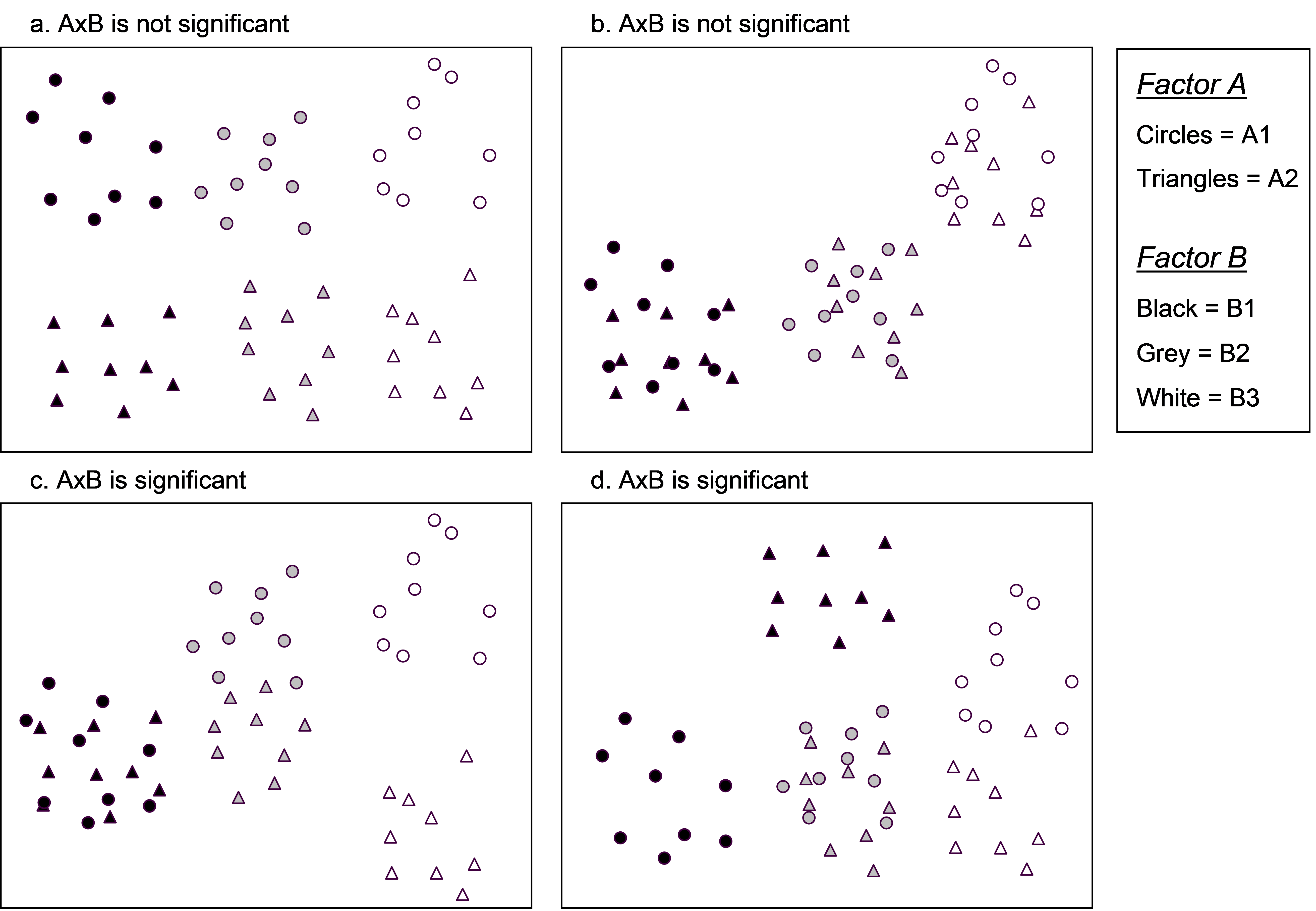 Fig. 1.17. Two-dimensional examples of two-way crossed designs in which: (a) effects of A occur in a similar direction and are of a similar magnitude within each level of B, and vice versa; (b) A apparently has no effects, while B has similar effects within each level of A; (c) effects of A depend on which level of B you are in, having either no effect (within B1), a clear effect (within B2) or a clear and large effect (within B3); and (d) interaction due to not just the size, but also the direction of the effects of A within each level of B.
To clarify ideas, consider a hypothetical two-way crossed experimental design with factor A having 2 levels (A1 and A2), factor B having 3 levels (B1, B2 and B3) and which can be drawn in two dimensions in Euclidean space (Fig. 1.17). We can conceive of a situation where the effect (shift in location) due to factor A (e.g., from triangles to circles) is of a similar size and in a similar direction, regardless of which level of factor B we happen to be in (Fig. 1.17a). In this case, there is no interaction. Similarly, we can conceive of a situation where there are apparently no effects of factor A at all, regardless of factor B, which would also result in there being no significant interaction (Fig. 1.17b). In contrast, we can conceive of situations where the sizes (or directions) of factor A’s effects are different within different levels of factor B (Fig. 1.17c, d). Note that, for univariate analysis, we consider changes in direction only along a single dimension for a given response variable, with an effect being either positive or negative. In contrast, there are many possible ways that changes in direction can happen in multivariate space.
The logic of the interpretation of a test for interaction in PERMANOVA follows, by direct analogy, the logic employed in univariate ANOVA. In particular, it is important to examine the test of the interaction term first in order to know how to proceed. As for univariate analysis, the presence of a significant interaction generally indicates that the test(s) of main effects (i.e., the test of each factor alone, ignoring the other factor) may not be meaningful. Appropriate logic dictates that the next step after obtaining a significant interaction is to do pair-wise comparisons for the factor of interest separately within each level of the other factor (i.e., to do pair-wise comparisons among levels of factor A within each level of factor B) and vice versa (if necessary). On the other hand, if the interaction term is not statistically significant, then this indicates effects (if any) of each factor do not depend on the other factor, and one may examine the individual pseudo-F tests of each factor alone (and do subsequent pair-wise comparisons, if appropriate), ignoring the other factor.
For the subtidal epibiotic assemblages, the lack of a significant interaction meant that we could logically proceed to investigate the main effects, which were each highly statistically significant. The next logical step is to consider pair-wise comparisons separately for each factor. For the factor of Position, there are only 2 levels, so the pseudo-F ratio demonstrates already that there is a significant difference between these two groups (near and far). (We might decide nevertheless to do pair-wise comparisons for this term, if we wish to know something more about the sizes of the average within-group or between-group dissimilarities, for example.) On the other hand, the factor of Shade has three levels and pair-wise comparisons are desirable to discern wherein the significant differences may lie (i.e., between which pairs of groups). Run the PERMANOVA routine again with all of the same choices in the dialog as for the main test, except this time choose (Test $\bullet$Pair-wise test > For term: Shade > For pairs of levels of factor: Shade) (Fig. 1.18). The results show that there is no significant difference between assemblages in the open and procedural control treatments (C, O), although both of these differed significantly from assemblages in the shade treatment (S) (Fig. 1.18).
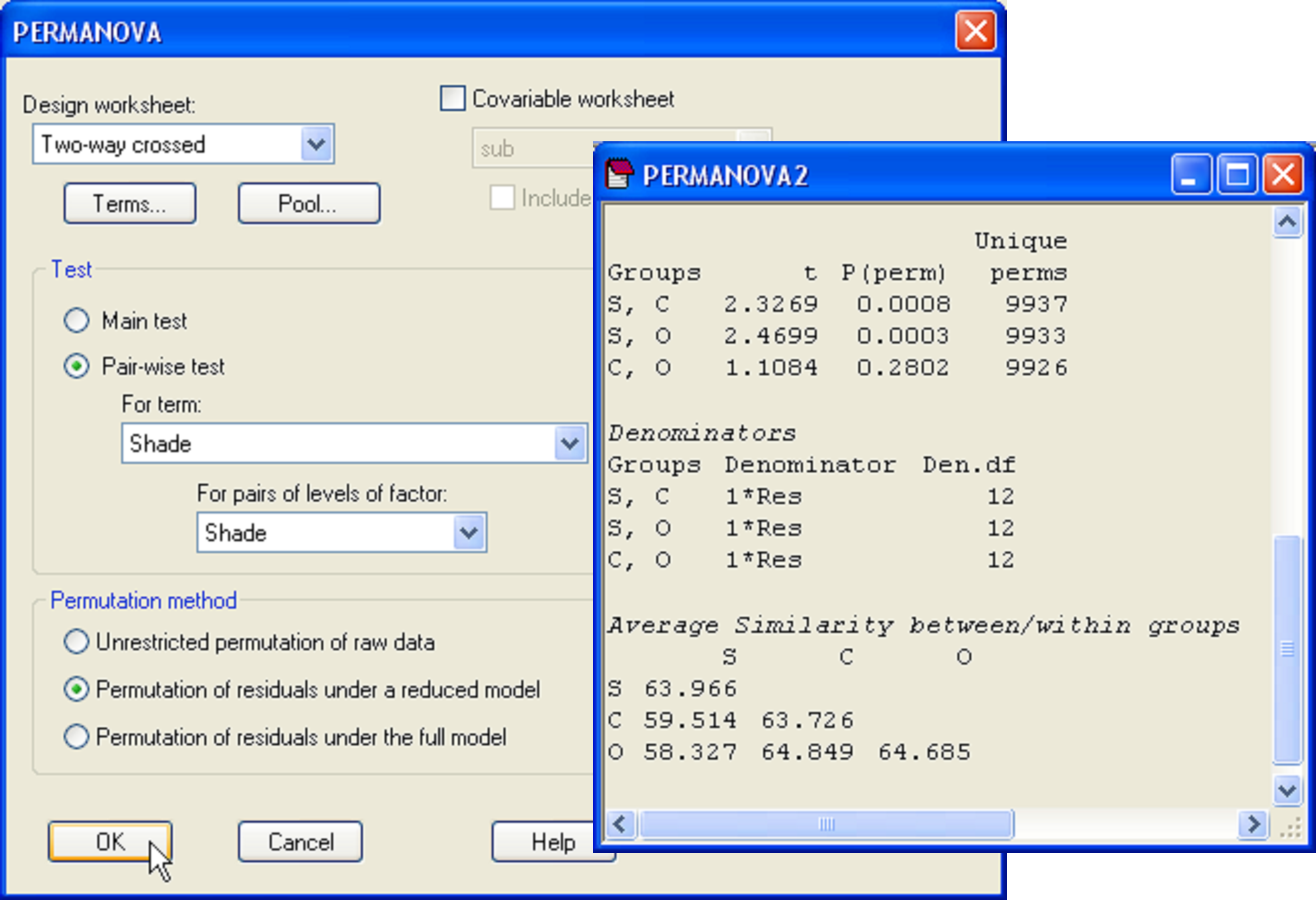 Fig. 1.18. PERMANOVA dialog and results for the comparison among the three shade treatments for subtidal epibiota.
In the event that the interaction term had been statistically significant, then the logical way to proceed would have been to do pair-wise tests among levels of the Shade factor separately for each of the near and far situations (i.e., within each level of factor Position). To do pair-wise comparisons like this, following on from an interaction term, one would choose (Test $\bullet$Pair-wise test > For term: PositionxShade > For pairs of levels of factor: Shade) in the PERMANOVA dialog. Similarly, one could also in that case consider doing comparisons among levels of the factor Position (near versus far) separately within each of the shade levels (S, O and C). For the latter, one would choose (Test $\bullet$Pair-wise test > For term: PositionxShade > For pairs of levels of factor: Position). In either case, one first chooses the interaction term of interest, followed by the particular factor involved in that interaction which is the focus for that set of pair-wise comparisons. In complex designs, there may be multiple sets of pair-wise comparisons that the user may wish to do in order to follow up the full model partitioning and results shown by the main test.
As a final note, keep in mind that the patterns in an MDS (or PCO) ordination plot may or may not show the reasons for an interaction, if it is present, because the full dimensionality of the multivariate cloud has been reduced (usually to 2 or 3 dimensions). Importantly, PERMANOVA works on the underlying dissimilarities themselves for the test, so its results should be trusted over and above any patterns (or lack of patterns) apparent in the ordination. Usually an ordination will help, however, to interpret the PERMANOVA results, provided the stress is not too high24.
23 It was noted earlier that PERMANOVA is not sensitive to differences in correlation structure among groups (Fig. 1.6). Similarly, the PERMANOVA test of interaction is focused more on the additivity of the sizes of the effects, rather than on their direction, per se. Thus, differences in effects which are directional but which do not affect the additivity of effect sizes may go undetected. Studies examining the power of PERMANOVA to detect different kinds of interactions are needed to clarify this issue further.
24 Stress is a measure of how well inter-point distances in an MDS ordination represent the rank-ordered inter-sample dissimilarities in the original resemblance matrix. For a more complete description of the notion of stress, see previous references to MDS along with chapter 5 of Clarke & Warwick (2001) and chapter 7 of Clarke & Gorley (2006) .