1.35 Designs with covariates (Holdfast invertebrates, revisited)
A topic that is related (perhaps surprisingly) to the topic of unbalanced designs is the analysis of covariance, or ANCOVA. There are some situations where the experimenter, faced with the analysis of a set of data in response to an ANOVA-type of experimental design, would like to take into account one or more quantitative variables or covariates. The essential idea here is that the response variable(s) may be known already to have a relationship with (or to be affected by) some (more or less continuous) quantitative variable. What is of interest then is to analyse the response data cloud given this known existing relationship. That is, one may wish to perform the ANOVA partitioning only after including (i.e., fitting, conditioning upon or taking into account) the covariate(s) in the model. Unfortunately, even if the design is completely balanced, so that terms are independent of one another, this is almost certainly not the case if a covariate is added to the model44. Thus, if one or more covariates are included in an ANOVA design (to yield what is commonly referred to as an ANCOVA model), the SS for individual terms in the model are not independent of one another. This means that the Type of SS must be chosen carefully for these situations, just as for an unbalanced case.
Generally, the covariate is to be fit first, with the design factors to be considered given the covariate, so there is a logical sequential order of terms. Thus, Type I SS usually makes the most sense here. However, using Type I SS does mean that the order of the fit of the design factors relative to each other will also matter, so this should be kept in mind. Thus, if Type I SS are to be used, the experimenter might also decide to re-run the analysis, swapping the order of factors in the ANOVA part of the model in order to check whether this affects any essential interpretations of the results. The order in which the individual terms are fit by PERMANOVA can be changed either by changing the order of the rows in the design file or by clicking on the ‘Terms…’ button in the PERMANOVA dialog to yield the ‘Ordered Selection’ window (e.g., Fig. 1.32), then using the up and down arrows to move the relative positions of individual terms that will be included in the sequential fit.
An example of a design which might include a covariate in the model is provided by the holdfast invertebrate dataset, seen in the section Nested design. It is known that the community structure of organisms inhabiting holdfasts is affected by the volume of the holdfast habitat itself (e.g., Smith, Simpson & Cairns (1996) ). This stands to reason, given the well-known ecological phenomenon of the species-area relationship (e.g., Arrhenius (1921) , Connor & McCoy (1979) ). Larger holdfasts have not only a larger colonisable area (which might alone be dealt with adequately through a standardisation by total sample abundance), but they also have greater complexity, usually with a greater number of interstices and root-like structures (called haptera) as well. The volume of each holdfast in the study by Anderson, Diebel, Blom et al. (2005) was measured using water displacement, and should really be included as a covariate in the analysis.
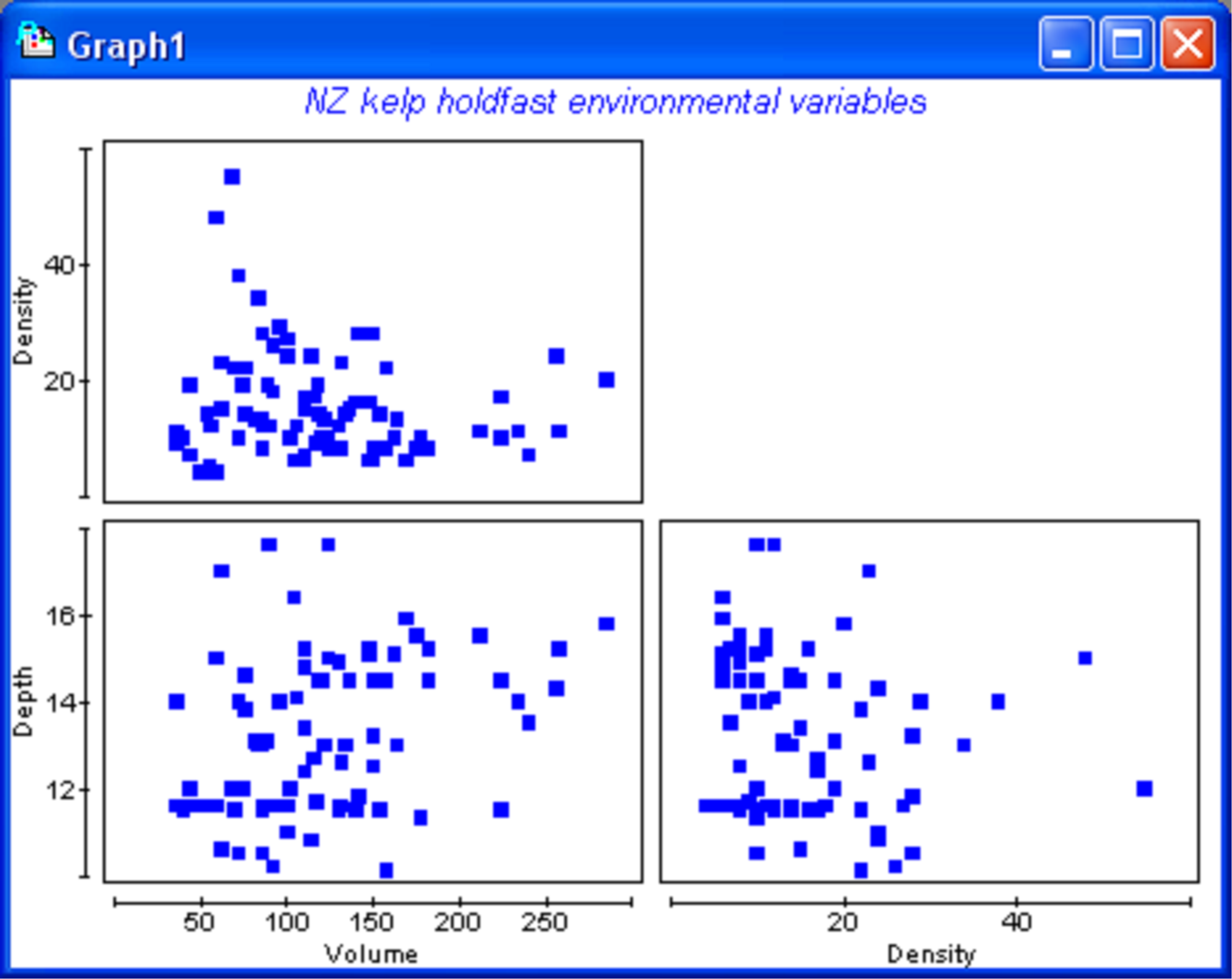
Fig. 1.45. Draftsman plot of environmental variables for kelp holdfasts.
Open up the file hold.pri in the folder ‘HoldNZ’ of the ‘Examples add-on’ directory. Here, we shall analyse only those species (or taxa) that occurred as counts of abundances. We will not include the encrusting organisms that were recorded only as an ordinal measure from 0-3. Choose Select > Variables > Indicator levels > Indicator name: Ordinal > Levels… > (Available Y) & (Include N). Choose Tools > Duplicate and re-name the data file produced as hold.abund. We shall base the analysis on a dissimilarity measure that is a modification of the Gower measure, recently described by Anderson, Ellingsen & McArdle (2006) . This measure is interpretable as the average order-of-magnitude difference in abundance per species, where each change in order of magnitude (i.e. 1, 10, 100, 1000 on a log10 scale) is given the same weight as a change in composition from 0 to 1 (see Anderson, Ellingsen & McArdle (2006) for more details). Choose Analyse > Resemblance > (Analyse between •Samples) & (Measure •More (tab)), click on the tab labeled ‘More’ and choose (•Others: Modified Gower > Modified Gower log base: 10). Save the current workspace as hold_cov.pwk.
Environmental data, including depth (in m), density of kelp plants where the holdfast was collected (per m2) and a measure of volume for each holdfast (in ml), are located in the file holdenv.pri, also located in the ‘HoldNZ’ folder. Open up this file within the hold_cov workspace just created and choose Analyse > Draftsman plot to examine the distributions of these environmental variables, focusing on the variable of ‘Volume’ in particular (Fig. 1.45). The distributions of environmental or other quantitative variables to be included as covariates in PERMANOVA should be investigated before proceeding. There are two important reasons for doing this:
-
The model fit by PERMANOVA is linear with respect to the covariate. That is, the relationship between the covariate and the multivariate community structure as represented in the space defined by the dissimilarity measure chosen is linear. Importantly, the relationship between the covariate and the original species (or other response) variables is emphatically not linear unless Euclidean distance is used as the basis of the analysis. So, the experimenter should look (as far as possible) for outliers and other oddities in the multivariate space of the dissimilarity measure chosen (i.e., using ordination) and should also examine the distribution of the covariate as part of a general diagnostic process before proceeding.
-
Permutation of raw data will have inflated type I error if there are outliers in the covariates ( Kennedy & Cade (1996) , Anderson & Legendre (1999) , Anderson & Robinson (2001) ). Thus, permutation of raw data is not allowed as an option if covariates are included in the PERMANOVA model.
If the distribution of the covariate is skewed or bimodal, then the user may wish either to transform the variable, or to split the dataset according to any clear modalities observed. See chapter 10 of Clarke & Gorley (2006) regarding the diagnostic process for interpreting and using draftsman plots for environmental variables. The main point is that covariates used in PERMANOVA should show approximately symmetric distributions that are roughly normal, with no extreme outliers. As pointed out by Clarke & Gorley (2006) , it is not necessary to agonise over this issue! Normality is by no means an assumption of the analysis, but outliers can have a strong influence on results. A draftsman plot of the holdfast environmental variables indicates that the distribution of volumes is fairly even, with no obvious skewness or outliers (Fig. 1.45), so no transformation is necessary.
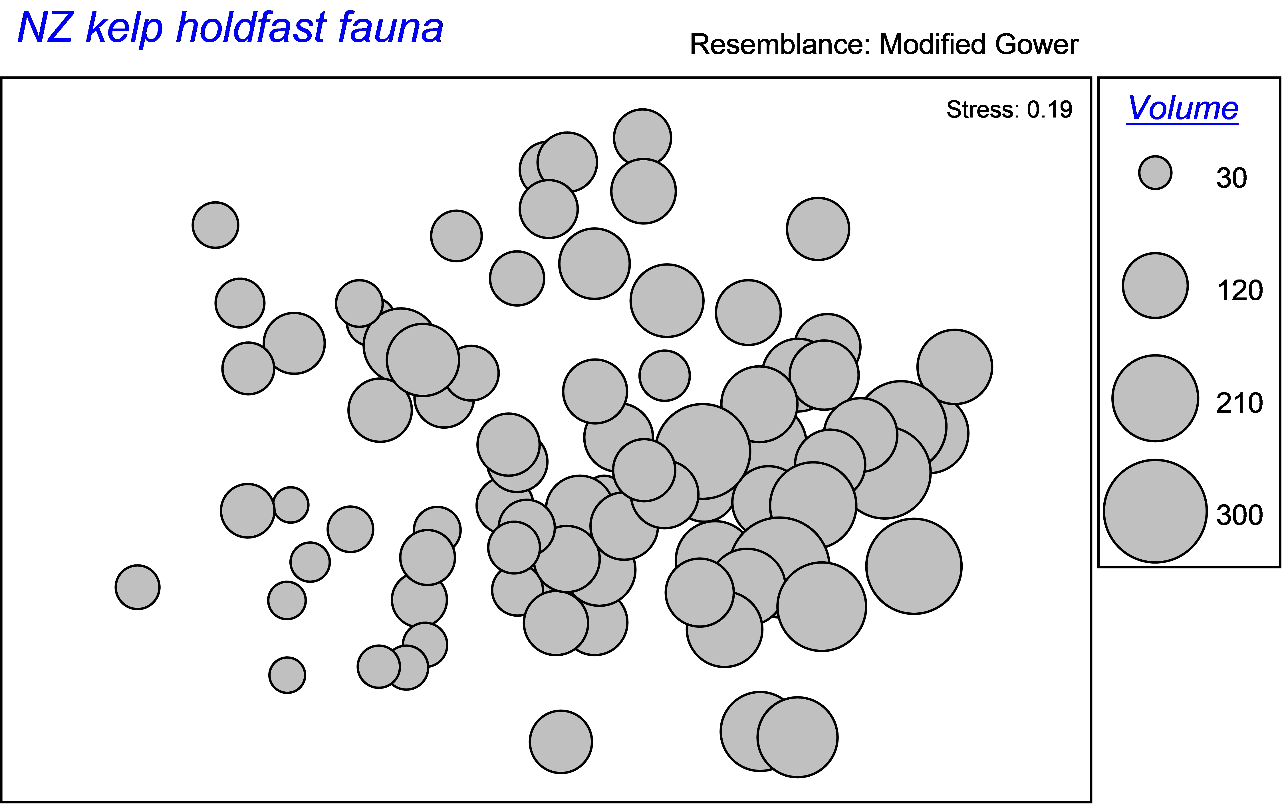
Fig. 1.46. MDS of holdfast fauna with volume superimposed as bubbles.
An MDS plot of the holdfast fauna with volume superimposed (as bubbles) shows a clear relationship between volume and community structure (Fig. 1.46); change in community structure from left to right across the diagram is associated with increasing volume of the holdfast. Thus, it would make sense to examine the variability in community structure at different spatial scales over and above this existing relationship with volume.
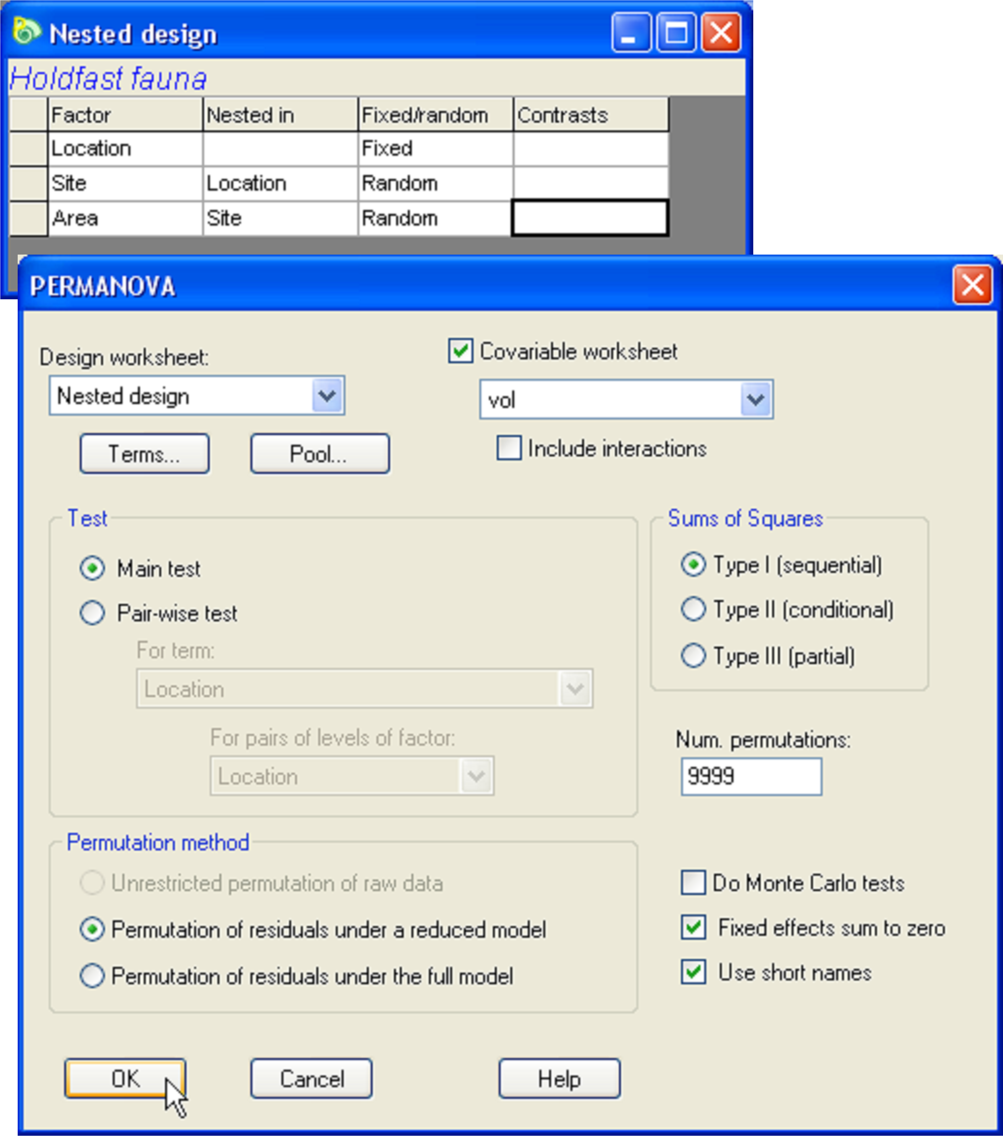
Fig. 1.47. PERMANOVA dialog for the analysis of holdfast fauna in response to the fully nested design and including volume as a covariate.
To proceed with the analysis, start by selecting the holdenv worksheet, highlight the single variable of Volume, choose Select >Highlighted followed by Tools >Duplicate, then re-name the resulting worksheet vol. It is important that the variable(s) to be used as covariate(s) in the model be contained in a single separate datasheet. It is also important that the labels of the samples in this data sheet match those that are contained in the resemblance matrix, although the particular order of the samples need not be the same in the two files. (PERMANOVA, like other routines in PRIMER, uses a label matching procedure to ensure correct analysis). Next, go to the Modified Gower resemblance matrix calculated from the hold.abund data sheet and create a PERMANOVA design file with three factors: Location, Site and Area, according to the fully nested design outlined in the section Nested design (e.g., Fig. 1.29). Re-name this design file Nested design. Click on the dissimilarity matrix again and choose PERMANOVA+ > PERMANOVA > (Design worksheet: Nested design) & (Covariable worksheet: vol) & (Sums of Squares •Type I SS (sequential)) & (Num. permutations: 9999) & (Permutation method •Permutation of residuals under a reduced model) & ($\checkmark$Use short names), as shown in Fig. 1.47.
The results of this analysis show that there is a strong and significant effect of the covariate, i.e., a significant relationship between holdfast volume and community structure as measured by the Modified Gower dissimilarity measure (Fig. 1.48). This is not surprising, given the pattern seen in the MDS plot (Fig. 1.46). Nevertheless, even given the variation among holdfast communities due to volume, significant variability is still detected among the assemblages at each spatial scale in the design: among locations (100’s of km’s), sites (100’s of m’s) and areas (10’s of m’s) (Fig. 1.48).
It is possible, in such an analysis, to include interactions between the covariate and each of the other terms in the experimental design. A significant interaction between a factor (such as Locations) and a covariate (such as volume) indicates that the nature of the relationship between the covariate and the multivariate responses differs within different levels of the factor (i.e., that the relationship between volume and holdfast community structure differs at different locations, and so on for other factors in the model). In the case of univariate data with a single factor and one covariate, as analysed in a traditional ANCOVA model, the test of the interaction term between the covariate and the factor is also known as a test for homogeneity of slopes. Sometimes ANCOVA is presented as a model without the interaction term and in these cases it is stated that homogeneity of slopes is an assumption of the analysis. However, if one includes the interaction term in the model, then clearly this type of homogeneity is no longer an assumption, as the model explicitly allows for different slopes for different levels of the factor. See Winer, Brown & Michels (1991) or Quinn & Keough (2002) for more complete discussions and examples of traditional ANCOVA models.
In PERMANOVA, tick the box labeled ‘Include interactions’ in the dialog under the specification of the covariable worksheet in order to include these terms in the model. Note that, after ticking this box, you can also still click on the ‘Terms…’ button and change the order in which the terms are fitted and/or exclude particular terms from the model if you wish, whether these be interactions with the covariate or some other terms. An analysis of the holdfast data where interaction terms are included suggests there is actually no compelling reason to include any of these interactions in the model in this particular case (P > 0.18 for all interactions with the covariate, Fig. 1.48).
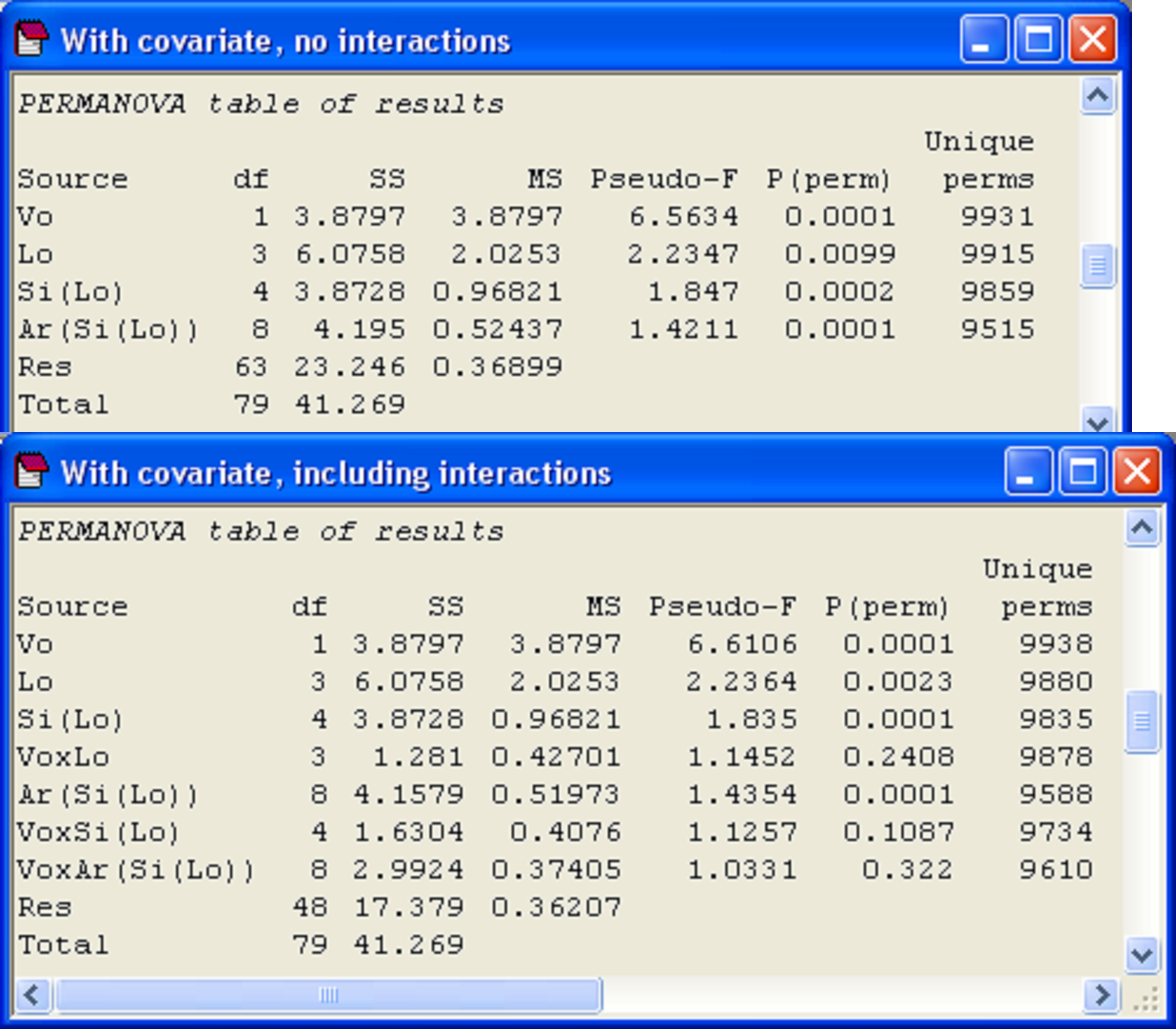 Fig. 1.48. PERMANOVA results of the analysis of holdfast fauna, including volume as a covariate, either (a) without interactions or (b) including interactions.
We re-iterate that the most important thing to remember about analyses involving covariates is that the individual terms are not independent of one another, so the Type of SS chosen for the analysis will affect the results, just as it does for unbalanced designs. What is more, the underlying complexity of this particular analysis45 (even without including the interaction terms), which is a mixed model having both random factors and a (fixed) covariate, can be appreciated by considering the EMS’s and the rather impressive gymnastics the program must go through in order to produce tests of individual terms using pseudo-F (Fig. 1.49). For more details on how these pseudo-F ratios were constructed, see the next section, Linear combinations of MS.
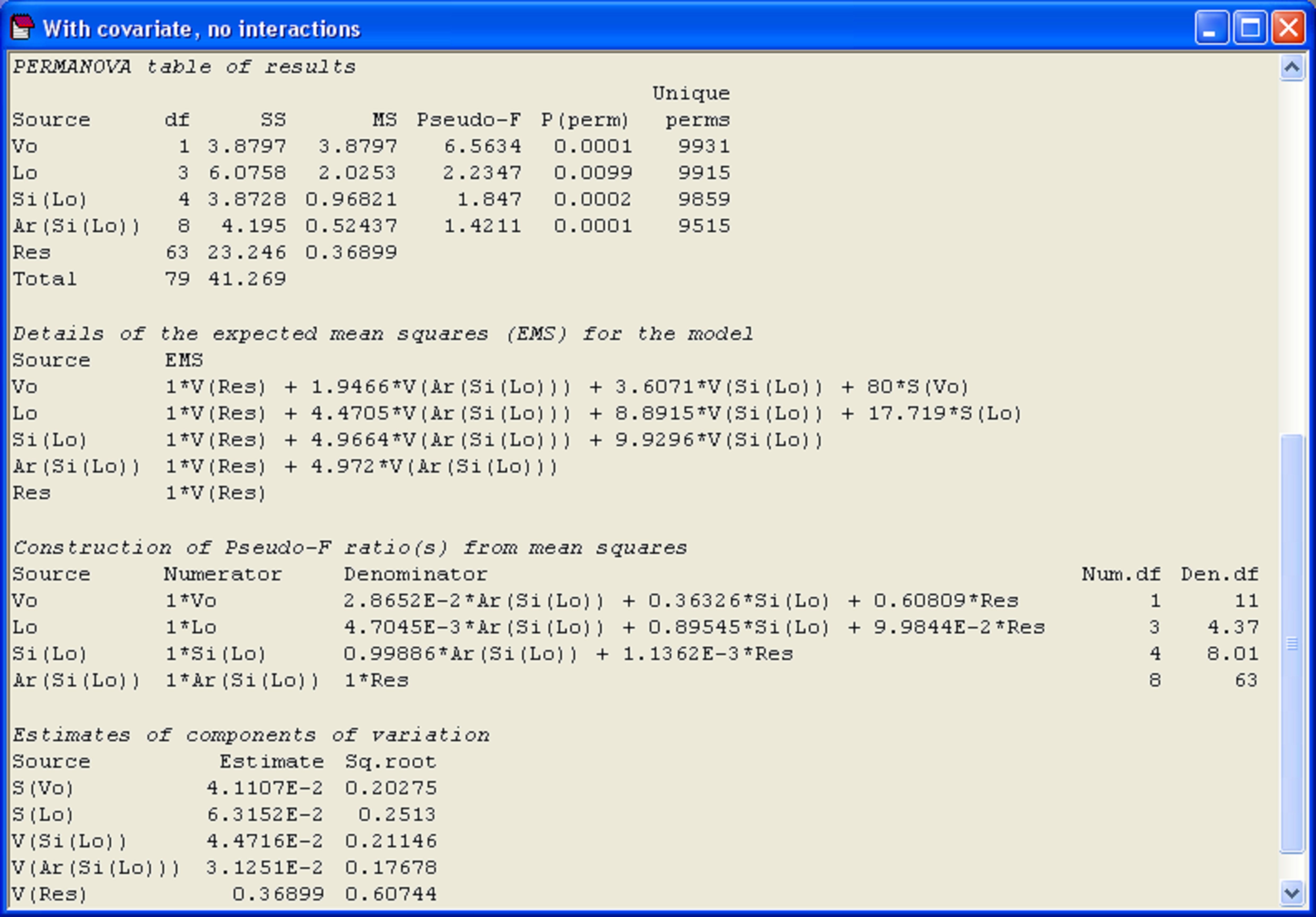
Fig. 1.49. PERMANOVA results of the analysis of holdfast fauna, including volume as a covariate and showing the EMS, construction of pseudo-F and components of variation for each term in the model.
44 The reason non-independence is introduced becomes clearer perhaps when we consider that if the covariate is fitted first and different ranges of the continuous covariate occur in different cells, then it cannot be independent of existing factors.
45 This complexity was, unfortunately, not recognised by the authors of the original paper ( Anderson, Diebel, Blom et al. (2005) ). The analyses they presented took a “naïve” view and conditioned on the covariate without considering the effects this would have on the EMS’s and pseudo-$F$ ratios for the other factors in the model. Making mistakes is, however, part of doing science and we would be nowhere if we did not make mistakes, acknowledge our errors and learn from them!