1.32 Repeated measures (Victorian avifauna, revisited)
While randomised blocks, latin squares and split-plot designs lack spatial replication, a special case of a design lacking temporal replication (and which occurs quite a lot in ecological sampling) is the repeated measures design (e.g., Gurevitch & Chester (1986) , Green (1993) ). In essence, these designs consist of individual sampling units (usually belonging to various treatments, etc.) which are repeatedly examined at several different time points. Such designs receive special attention for two reasons: (i) they do not have replication within cells, so suffer from the same issues discussed in the previous two sections and (ii) they require some additional assumptions because samples are generally considered to be non-independent through time. The first issue – lack of replication – is dealt with easily enough by PERMANOVA, as discussed above. The program (after issuing the usual warning) will simply exclude the highest-order interaction term (i.e. which will include “Time” as one of its members) and the analysis proceeds from there in the usual way.
The issue of non-independence is, however, another matter. In a traditional repeated measures analysis of univariate data, the partitioning of the total sum of squares is done in the usual way, treating “Time” as a fixed factor. What is taken on as an additional assumption, however, is something known as sphericity. Sphericity is an assumption about the nature of the correlations through time for the sample units, which must be similar for the different treatments. Although a formal test of sphericity is provided by Mauchley (1940) (see Winer, Brown & Michels (1991) for an example), this approach is unfortunately rather highly susceptible to deviations from normality ( Huyhn & Mandeville (1979) ). Huynh & Feldt (1970) have demonstrated that a necessary and sufficient condition is to check the equality of the variances of the differences between levels of the repeated measures factor (“Time”) across treatments (or combinations of treatments). Thus, one calculates the differences between each pair of time points, obtains the variances of these difference values for each treatment (or treatment combination) and then checks for equality of these variances (e.g., Quinn & Keough (2002) ). If this assumption is violated, then the F ratios obtained from the analysis are no longer distributed like traditional F distributions under true null hypotheses. In this case, for traditional univariate analysis, a number of possible corrections to the degrees of freedom can be done to get a correct test (e.g., Box (1954) , Geisser & Greenhouse (1958) , Huynh & Feldt (1976) ).
When dealing with multivariate response data, one might consider doing an analogous test of sphericity (of some sort) by calculating the dissimilarities (or distances) between levels of the repeated measures factor across treatments. The variances of these dissimilarities could then be compared among treatments (or treatment combinations) using, for example, PERMDISP (see chapter 2), or even using a traditional test for homogeneity of variances among groups.
Recall, however, that PERMANOVA uses permutation procedures in order to generate a correct distribution of each pseudo-F statistic under a (relevant) true null hypothesis. So the only essential assumption associated with the use of PERMANOVA (whether there be repeated measures or otherwise) is the exchangeability of samples (or of appropriate residuals). It must be admitted that the correlation structure among samples through time, if any, will be effectively ignored under permutation. Thus, differences in correlation structure through time among treatments (i.e. lack of sphericity) may, therefore, produce a statistically significant result. However, we consider that differences in correlation structure through time are indicative of (at least one type of) a treatment effect, so should warrant closer inspection by the investigator in any event.
Clearly, the degree to which correlation structure (in space or in time, as in repeated measures) can affect the results of permutation tests for repeated measures designs (or any other designs for that matter) warrants further study. If statistically significant results are obtained in a repeated measures analysis, the user may wish to accompany the PERMANOVA with a separate test for sphericity (in the case of univariate data) or its analogue (using dissimilarities rather than differences) for multivariate responses, in order to shed further light on the meaning of the results and appropriate inferences.
An example helps to clarify these ideas. The data on Victorian avifauna, previously examined in the section Monte-Carlo P-values, actually consisted of a repeated measures design, as described by Mac Nally & Timewell (2005) . The previous analyses (Figs. 1.12 and 1.13) were based on data summed across four different observation times. However, these data are also available at the level of individual surveys done at each time in the file vicsurv.pri in the folder ‘VictAvi’ of the ‘Examples add-on’ directory. Open up the data and calculate the dissimilarity matrix among samples on the basis of the binomial deviance dissimilarity measure; re-name this matrix BinomDev.
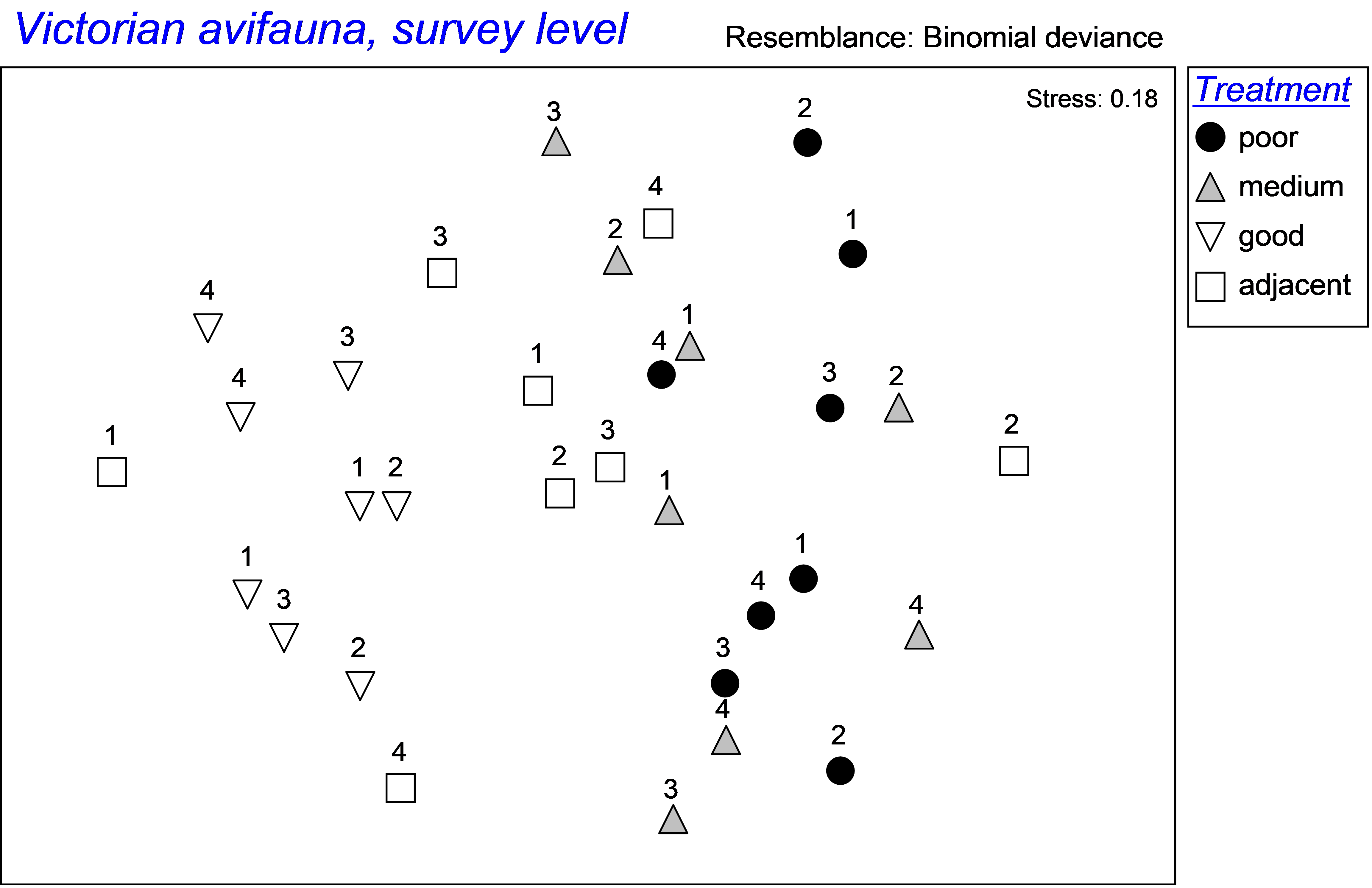
Fig. 1.38. MDS of Victorian avifauna at each of two sites within each of several states of flowering intensity (poor, medium, good or adjacent to a good site) for 4 times (given as numbers on the plot).
An MDS ordination on the basis of this matrix suggests a strong effect of flowering intensity on the bird communities, with ‘good’ sites appearing to the left of the diagram, ‘poor’ or ‘medium’ sites occurring to the right, and ‘adjacent’ samples being more variable than the other treatments through time (Fig. 1.38). The repeated measures experimental design here is:
Factor A: Treatment (fixed with a = 4 levels: poor, medium, good or adjacent).
Factor B: Site (random, nested in Treatments with b = 2 levels, labeled simply S1-S8).
Factor C: Time (fixed40 with c = 4 levels, labeled 1-4).
After creating the design file, re-name it Repeated measures for reference. Note that there is no replication within cells, as there is only one sample per site at each time. We therefore need to exclude the highest-order interaction, ‘Site(Treatment) × Time’, from the model. See Fig. 1.39 and refer to the above section Pooling or excluding terms, if necessary, for details on how to do this. Analysis by PERMANOVA (with 9999 permutations of residuals under a reduced model) reveals significant treatment effects on the bird assemblages (Fig. 1.39), and shows that these effects are consistent through time (note that P > 0.6 for ‘TrxTi’). Pair-wise comparisons (not shown here, but you can do them easily) reveal that this effect is largely due to there being significant differences between the good sites vs the others.
Having identified significant treatment effects, we may wish to examine the multivariate analogue to the test of sphericity for univariate data. Namely, we can calculate the dissimilarities between each pair of time points within each treatment. Then, we can compare the time-point differences for equality of variances. This is purely optional and is not a requirement of the repeated measures analysis when performed using PERMANOVA, but it may nevertheless shed some further light on whether the significant treatment effects detected were due only to differences in location in multivariate space (as would appear to be the case from the diagram) or whether sites might also vary in the nature of their non-independence among time points.
To do this, we first need to extract the relevant dissimilarities between time-points for each sampling unit (in this case, from each site) from the full dissimilarity matrix. These are shown in Table 1.4. For example, the binomial deviance dissimilarity between times 1 and 2 for site 1 (a ‘poor’ site) is 17.85, and so on. These multivariate dissimilarity values can take on the same role as the differences among time points which are usually examined in a univariate repeated measures analysis (e.g., see Box 10.6 in Quinn & Keough (2002) )41. The estimated variances in these dissimilarities (given in the last row of Table 1.4) appear to be similar among the six paired groups (i.e. the six columns in Table 1.4). Levene’s test (using either means $F _{5,42} = 0.59$, P > 0.71 or medians $F _{5,42} = 0.32$, P > 0.90), supports the assumption of homogeneity of these variances42. This means we can fairly safely infer in this case that the treatment effects we detected were not caused by differences in dissimilarity structure within samples through time among the sites43.
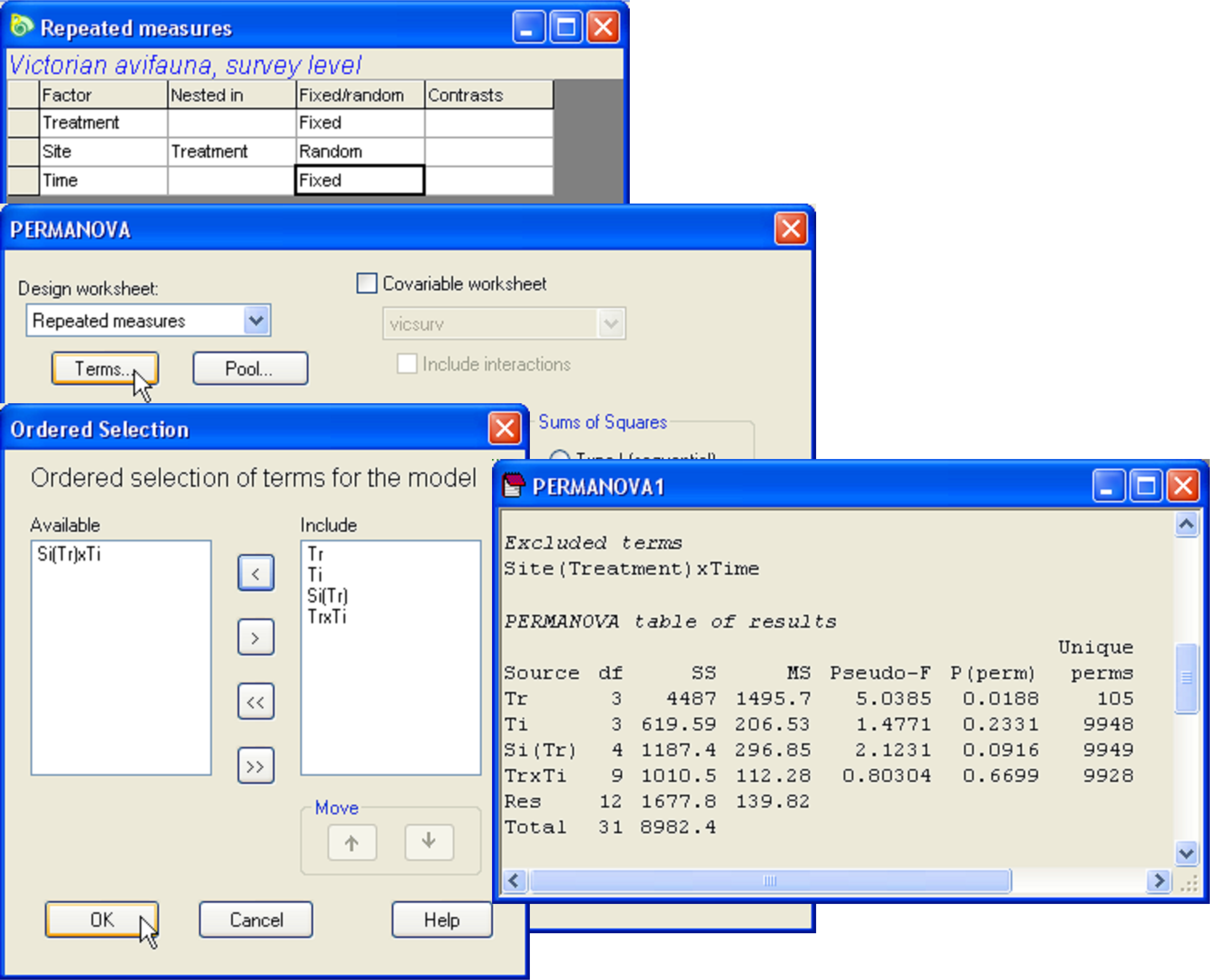
Fig. 1.39. PERMANOVA analysis of a repeated measures experimental design for Victorian avifauna.
Before leaving the topic of repeated measures, there is one other method of analysis worth mentioning. With univariate data, one has the option of treating the individual values at each time point as separate variables, then doing a multivariate analysis among treatments. Note that this approach will only work when there is one response variable measured at different times. It is to be distinguished from the situation we have above, where there are already multivariate data (i.e., abundances of 27 species of birds) obtained at each time point. The multivariate approach to a repeated measures analysis of a single response variable is, however, straightforward to do using PERMANOVA – one simply organises the data so that measures at different time points are the “variables” and uses Euclidean distance as the basis of the analysis. Although taking a multivariate approach with univariate data (treating the time points as variables) completely avoids having to consider any notions of sphericity, it does not provide any test of the factor ‘Time’ or any tests of the interactions of ‘Time’ with (most) other factors, which would, of course, be provided by a traditional repeated measures partitioning. Green (1993) discusses other pros and cons with using the multivariate versus the univariate approach to a repeated measures analysis of a single variable (see Fig. 6 therein).
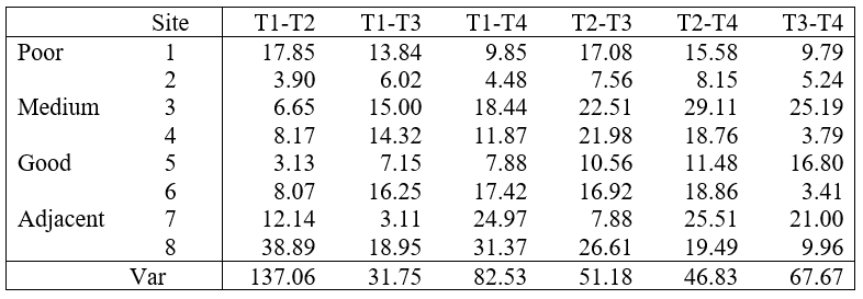
Table 1.4. Binomial deviance dissimilarities between time points for each site and their estimated variances.
For repeated measures designs and in other cases where there is known to be correlation structure (non-independence) among replicates, there may be other ways to analyse the data. First, one might consider rephrasing hypotheses in terms of dissimilarities between particular pairs of correlated objects, then analysing those dissimilarities in a univariate analysis. For example, Faith, Humphrey & Dostine (1991) tested the null hypothesis of no difference in the average dissimilarity between an impact and a control site from before to after the onset of a disturbance (with individual time points treated as replicates). Similarly, if one has a baseline or control against which other treatments are to be compared through time, one might consider using principal response curves (PRC, van den Brink & ter Braak (1999) ), which is simply a special form of redundancy analysis (RDA) .
Distance-based redundancy analysis (dbRDA) can also be used to model changes in the community through time (or space) explicitly as a linear, quadratic or other polynomial traveling through the multivariate data cloud (e.g. Makarenkov & Legendre (2002) ), rather than treating time (or space) as an ANOVA factor (see the chapters on DISTLM and dbRDA below for more details). Larger-scale monitoring programs, which generally have many sites sampled repeatedly at many times, can also be analysed using multivariate control charts ( Anderson & Thompson (2004) ). This approach is designed to detect when (and where) individual sites deviate significantly from what would be expected, given natural temporal variability.
40 We have chosen to treat “Time” as a fixed factor here, because this is traditionally how it is treated in repeated measures experimental designs. However, the user can of course choose to treat this factor as random if this is more in line with relevant hypotheses of interest.
41 Bear in mind that the univariate differences, however, can show direction by being either positive or negative, which will affect calculated variances. In contrast, dissimilarities are always positive, so cannot show direction, per se. Therefore, this is not at all intended to be a strict test for sphericity, merely to provide a means of examining the null hypothesis of no difference in dissimilarity structure among time points for individual samples across the different treatments. See also the approach used by Clarke, Somerfield, Airoldi et al. (2006) .
42 Note the use of a traditional univariate Levene’s test here for testing homogeneity of variances. We could also have done this test using a permutational approach in the routine PERMDISP on the basis of a Euclidean distance matrix for the univariate variable produced in Table 1.1. Indeed, if the tables are used, then this is equivalent to doing a traditional Levene’s test. See the chapter on PERMDISP for more details.
43 Winer, Brown & Michels (1991) discuss how correlations may need to be examined at several different levels in more complex multi-factorial repeated measures designs (see chapter 7 therein). We do not pursue this further here.