3.3 Mechanics of PCO
To construct axes that maximise fitted variation (or minimise residual variation) in the cloud of points defined by the resemblance measure chosen, the calculation of eigenvalues (sometimes called “latent roots”) and their associated eigenvectors is required. It is best to hold on to the conceptual description of what the PCO is doing and what it produces, rather than to get too bogged down in the matrix algebra required for its computation. More complete descriptions are available elsewhere (e.g., Gower (1966) , Legendre & Legendre (1998) ), but in essence, the PCO is produced by doing the following steps (Fig. 3.1):
- From the matrix of dissimilarities, D, calculate matrix A, defined (element-wise) as minus one-half times each dissimilarity (or distance)63;
- Centre matrix A on its row and column averages, and on the overall average, to obtain Gower’s centred matrix G;
- Eigenvalue decomposition of matrix G yields eigenvalues ($\lambda _ i$ , i = 1, …, N) and their associated eigenvectors.
- The PCO axes Q (also called “scores”) are obtained by multiplying (scaling) each of the eigenvectors by the square root of their corresponding eigenvalue64.
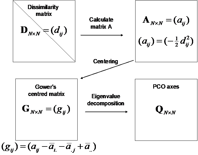
Fig. 3.1. Schematic diagram of the mechanics of a principal coordinates analysis (PCO).
The eigenvalues associated with each of the PCO axes provide information on how much of the variability inherent in the resemblance matrix is explained by each successive axis (usually expressed as a percentage of the total). The eigenvalues (and their associated axes) are ordered from largest to smallest, and their associated axes are also orthogonal to (i.e., perpendicular to or independent of) one another. Thus, $\lambda _ 1$ is the largest and the first axis is drawn through the cloud of points in a direction that maximises the total variation along it. The second eigenvalue, $\lambda _ 2$, is second-largest and its corresponding axis is drawn in a direction that maximises the total variation along it, with the further caveat that it must be perpendicular to (independent of) the first axis, and so on. Although the decomposition will produce N axes if there are N points, there will generally be a maximum of N – 1 non-zero axes. This is because only N – 1 axes are required to place N points into a Euclidean space. (Consider: only 1 axis is needed to describe the distance between two points, only 2 axes are needed to describe the distances among three points, and so on…). If matrix D has Euclidean distances to begin with and the number of variables (p) is less than N, then the maximum number of eigenvalues will be p and the PCO axes will correspond exactly to principal component axes that would be produced using PCA.
The full set of PCO axes when taken all together preserve the original dissimilarities among the points given in matrix D. However, the adequacy of the representation of the points as projected onto a smaller number of dimensions is determined for a PCO by considering how much of the total variation in the system is explained by the first two (or three) axes that are drawn. The two- (or three-) dimensional distances in the ordination will underestimate the true dissimilarities65. The percentage of the variation explained by the ith PCO axis is calculated as ($100 \times \lambda _ i / \sum \lambda _ i $). If the percentage of the variation explained by the first two axes is low, then distances in the two-dimensional ordination will not necessarily reflect the structures occurring in the full multivariate space terribly well. How much is “enough” for the percentage of the variation explained by the first two (or three) axes in order to obtain meaningful interpretations from a PCO plot is difficult to establish, as it will depend on the goals of the study, the original number of variables and the number of points in the system. We suggest that taking an approach akin to that taken for a PCA is appropriate also for a PCO. For example, a two-dimensional PCO ordination that explains ~70% or more of the multivariate variability inherent in the full resemblance matrix would be expected to provide a reasonable representation of the general overall structure. Keep in mind, however, that it is possible for the percentage to be lower, but for the most important features of the data cloud still to be well represented. Conversely, it is also possible for the percentage to be relatively high, but for considerable distortions of some distances still to occur, due to the projection.
63 If a matrix of similarities is available instead, then the PCO routine in PERMANOVA+ will automatically translate these into dissimilarities as an initial step in the analysis.
64 If the eigenvalue ($\lambda _ i$) is negative, then the square root of its absolute value is used instead, but the resulting vector is an imaginary axis (recall that any real number multiplied by $i = \sqrt{-1}$ is an imaginary number).
65Except in certain rare cases, where the first two or three axes might explain greater than 100% of the variability! See the section on Negative eigenvalues.