3.7 PCO versus PCA (Clyde environmental data)
Principal components analysis (PCA) is described in detail in chapter 4 of Clarke & Warwick (2001) . As stated earlier, PCO produces an equivalent ordination to a PCA when a Euclidean distance matrix is used as the basis of the analysis. Consider the environmental data from the Firth of Clyde ( Pearson & Blackstock (1984) ), as analysed using the PCA routine in PRIMER in chapter 10 of Clarke & Gorley (2006) . These data consist of 11 environmental variables, including: depth, the concentrations of several heavy metals, percent carbon and percent nitrogen found in soft sediments from benthic grabs at each of 12 sites along an east-west transect that spans the Garroch Head sewage-sludge dumpground, with site 6 (in the middle) being closest to the actual dump site. The data are located in the file clev.pri in the ‘Clydemac’ folder of the ‘Examples v6’ directory.
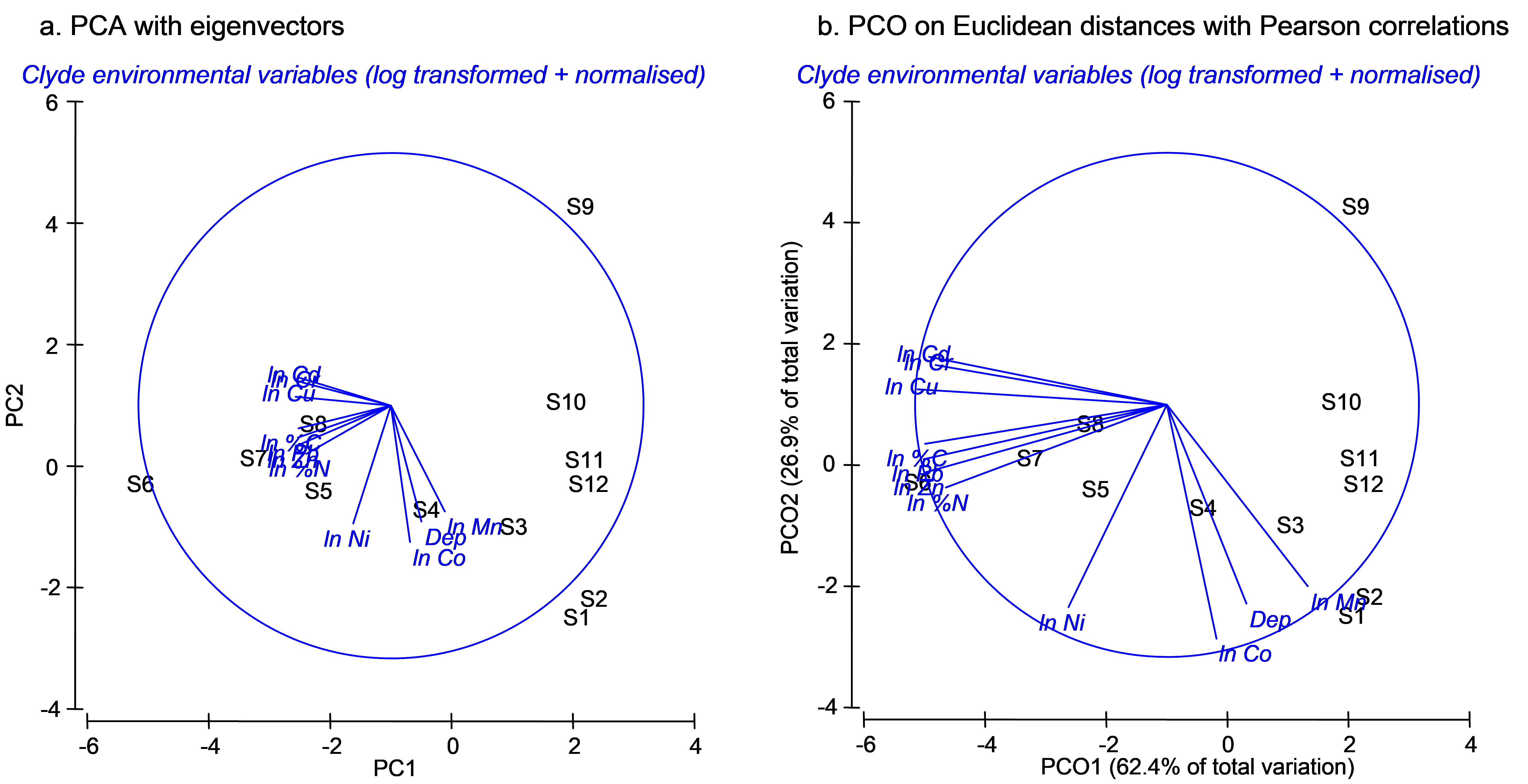 Fig. 3.9. Ordination of 11 environmental variables from the Firth of Clyde using (a) PCA and (b) PCO on the basis of a Euclidean distance matrix. Vectors in (a) are eigenvectors from the PCA, while vectors in (b) are the raw Pearson correlations of variables with the PCO axes.
As indicated by Clarke & Gorley (2006) , it is appropriate to first check the distributions of variables (e.g., for skewness and outliers) before proceeding with a PCA. This can be done, for example, by choosing Analyse>Draftsman Plot in PRIMER. As recommended for these data by Clarke & Gorley (2006) , log-transform all of the variables except depth. This is done by highlighting all of the variables except depth and choosing Tools > Transform(individual) > Expression: log(0.1+V) > OK. Rename the transformed variables, as appropriate (e.g. Cu can be renamed ln Cu, and so on), and then rename the data sheet of transformed data clevt. Clearly, these variables are on quite different measurement scales and units, so a PCA on the correlation matrix is appropriate here. Normalise the transformed data by choosing Analyse > Pre-treatment > Normalise variables. Rename the data sheet of normalised variables clevtn. Finally, do a PCA of the normalised data by choosing Analyse > PCA.
Recall that PCA is simply a centred rotation of the original axes and that the resulting PC axes are therefore linear combinations of the original (in this case, transformed and normalised) variables. The ‘Eigenvectors’ in the output file from a PCA in PRIMER provide explicitly the coefficients associated with each variable in the linear combination that gives rise to each PC axis. Importantly, the vectors shown on the PCA plot are these eigenvectors, giving specific information about these linear combinations. This means, necessarily, that the lengths and positions of the vectors depend on the other variables included in the analysis70.
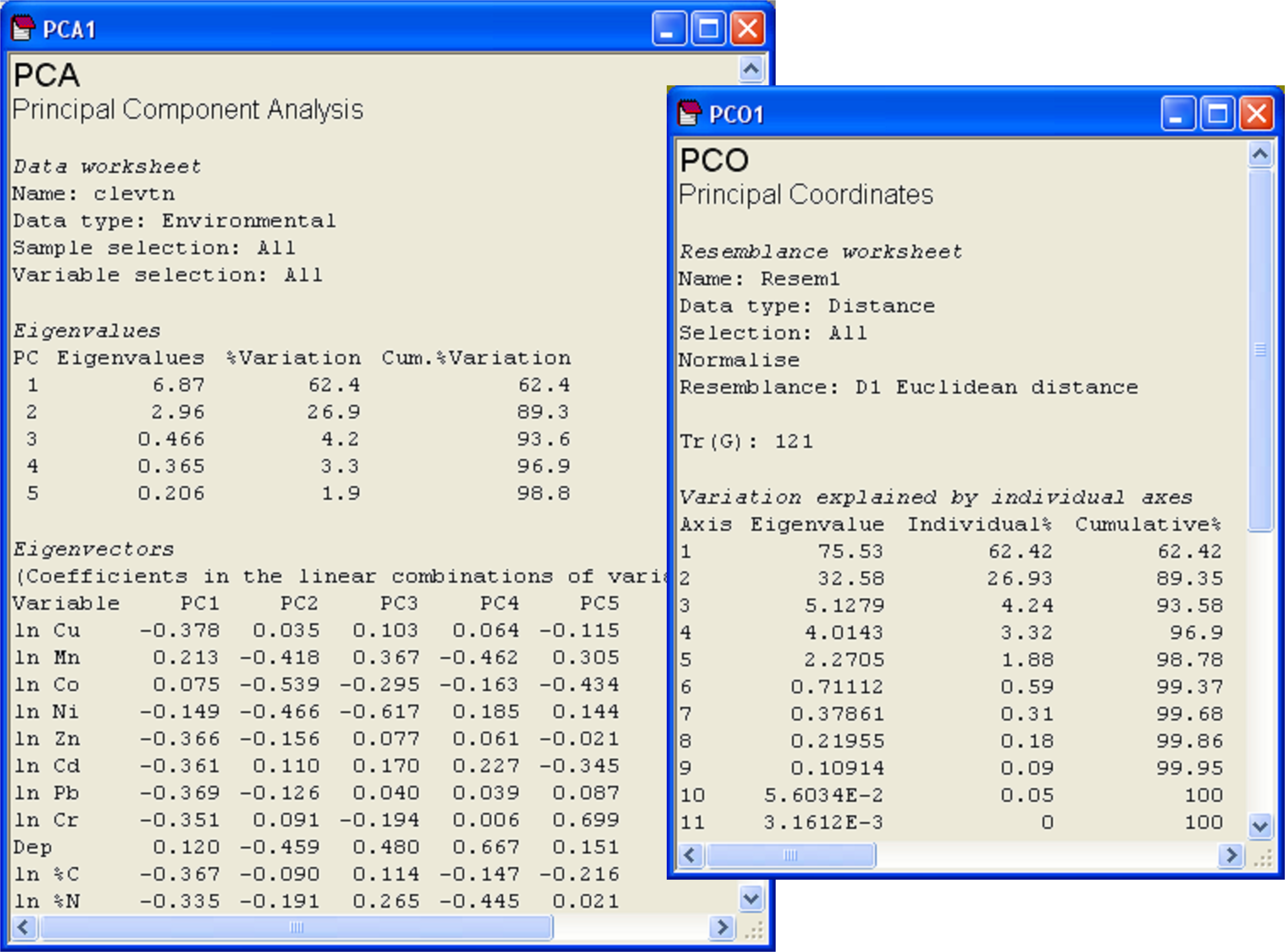
Fig. 3.10. Results of PCA and PCO on Euclidean distances for the transformed and normalised environmental data from the Firth of Clyde.
Next we may replicate the pattern of points seen in the PCA ordination precisely by doing a PCO on the basis of a Euclidean distance matrix. From the clevtn data file, choose Analyse > Resemblance > (Analyse between •Samples) & (Measure •Euclidean distance) > OK. From the resulting resemblance matrix, choose PERMANOVA+ > PCO > OK. For PCO, as for PCA, the sign of axes is arbitrary. It may be necessary to choose Graph > Flip X and/or Graph > Flip Y before the orientation of the PCO plot can be seen to match that of the PCA. Once this is done, however, it should be readily apparent that the patterns of points and even the scaling of axes are identical for these two analyses (Fig. 3.9). Further proof of the equivalence is seen by examining the % variation explained by each of the axes, as provided in the text output files (Fig. 3.10). The first two axes alone explain over 89% of the variation in these 11 environmental variables, indicating that the 2-d ordination is highly likely to have captured the majority of the salient patterns of variation in the multi-dimensional data cloud.
By choosing Graph > Special > (Vectors •Worksheet variables: clevtn > Correlation type: Pearson), vectors are drawn onto the PCO plot that correspond to the Pearson correlations of individual variables with the PCO axes. These are clearly different from the eigenvectors that are drawn by default on the PCA plot. For the vector overlay on the PCO plot, each variable was treated separately and the vectors arise from individual correlations that do not take into account any of the other variables. In contrast, the eigenvectors of the PCA do take into account the other variables in the analysis, and would obviously change if one or more of the variables were omitted. It is not surprising, in the present example, that log-concentrations of many of the heavy metals are strongly correlated with the first PCO axis, showing a gradient of decreasing contamination with increasing distance in either direction away from the dumpsite (site 6).
The PCA eigenvectors are not given in the output from a Euclidean PCO analysis. This is because the PCO uses the Euclidean distance matrix alone as its starting point, so has no “memory” of the variables which gave rise to these distances. We can, however, obtain these eigenvectors retrospectively, as the resulting PCO axes in this case coincide with what would be obtained by running a PCA – they are therefore linear combinations of the original (transformed and normalised) variables. This is done by choosing Graph > Special > (Vectors •Worksheet variables: clevtn > Correlation type: Multiple). What this option does is to overlay vectors that show the multiple partial correlations of the variables in the chosen worksheet with the configuration axes. In this case, these correspond to the eigenvectors. If you click on the option ‘Correlations to worksheet’ in the ‘Configuration plot’ dialog, you will see in this worksheet that the values for each variable correspond indeed to their eigenvector values as provided in the PCA output file71. This equivalence will hold provided variables have been normalised prior to analysis.
More generally, the relevant point here is that the choice of ‘Correlation type: Multiple’ will produce a vector overlay of multiple partial correlations, where the relationships between variables and configuration axes take into account other variables in the worksheet. This contrasts with the choice of ‘Correlation type: Pearson’ (or Spearman), which plot raw correlations for each variable, ignoring all other variables. For the PCA, note that it is also possible to replace the eigenvectors of original variables that are displayed by default on the ordination with an overlay of some other vectors of interest. This is done by simply choosing ‘•Worksheet variables’ and indicating the worksheet that contains the variables of interest, instead of ‘•Base variables’ in the ‘Configuration Plot’ dialog.
A further point to note is the fact that there are no negative eigenvalues in this example. Indeed, the cumulative scree plot for either a PCA or a PCO based on Euclidean distances will simply be a smooth increasing function from zero to 100%. Any measure that is Euclidean-embeddable and fulfils the triangle inequality will have strictly non-negative eigenvalues in the PCO and thus will have all real and no imaginary axes ( Torgerson (1958) , Gower (1982) , Gower & Legendre (1986) ).
If PCO is done on a resemblance matrix obtained using the chi-squared distance measure (measure D16 under the ‘Distance’ option under the ‘More’ tab of the ‘Resemblance’ dialog), then the resulting ordination will be identical to a correspondence analysis (CA) among samples that has been drawn using scaling method 1 (see p. 456 and p. 467 of Legendre & Legendre (1998) for details). Although the relationship between the original variables and the resulting ordination axes is linear for PCO on Euclidean distances (a.k.a. PCA) and unimodal for PCO on chi-squared distances (a.k.a. CA), when PCO is based on some other measure, such as Bray-Curtis, these relationships are likely to be highly non-linear and are generally unknown. Clearly, PCO is more general and flexible than either PCA or CA. This added flexibility comes at a price, however. Like MDS, PCO necessarily must lose any direct link with the original variables by being based purely on the resemblance matrix. Relationships between the PCO axes and the original variables (or any other variables for that matter) can only be investigated retrospectively (e.g., using vector overlays or bubbles), as seen in the above examples.
70This is directly analogous to the fact that the regression coefficient for a variable $X _1$ in the simple regression of $Y$ vs $X _1$, will be different from the partial regression coefficient in the multiple regression of $Y$ vs $X _1$ and $X _2$ together. That is, the relationship between $Y$ and $X _1$ changes once $X _2$ is taken into account. Correlation (non-independence) between $X _1$ and $X _2$ is what causes simple and partial regression coefficients to differ from one another.
71 The sign associated with the values given in this file and given for the eigenvectors will depend, of course, on the sign of the PCO and PCA axes, respectively, that happen to be provided in the output. As these are arbitrary, the signs may need to be “flipped” to see the concordance.