4.14 Analysing variables in sets (Thau lagoon bacteria)
In some situations, it is useful to be able to partition variability in the data cloud according to sets of predictor variables, rather than treating each variable individually. For example, Borcard, Legendre & Drapeau (1992) discussed the partitioning of variation in multivariate species data among two sets of variables: a set of environmental variables and a set of spatial variables (such as latitude and longitude, arbitrary spatial coordinates, or polynomial functions of these). They considered that analyses of the relationship between species data and environmental variables should include a consideration of the intrinsic spatial structuring caused simply by the relative geographic distances among samples at a given scale. One might expect, for example, that samples close together would be more similar than those further apart. By analysing the data in sets, one can explicitly examine the proportion of variation in the species data that is explained by the environmental variables over and above the amount explained by the spatial variables alone.
DISTLM can treat variables either individually or in sets. To identify sets of variables, one needs to first define an indicator which will identify the set that a particular predictor variable belongs to. Recall that an indicator in PRIMER identifies groups of variables the same way that a factor identifies groups of samples (see chapter 2 in Clarke & Gorley (2006) ).
As an example, we shall analyse a data set on the responses of heterotrophic bacteria grown in different media (labeled ‘Ma’ and ‘Bna’) to sets of environmental and spatial variables obtained from each of 20 sites in the Thau lagoon ( Amanieu, Legendre, Troussellier et al. (1989) ) provided by Legendre & Legendre (1998) (p. 529). Data on the bacteria are located in the file thbac.pri, and the associated environmental and spatial variables are located in the file thevsp.pri, both in the ‘Thau’ folder of the ‘Examples add-on’ directory. For the bacteria, the variable Bna is the concentration of colony-forming units of aerobic heterotrophs growing on bioMérieux nutrient agar (low salinity) and Ma is the concentration growing on marine agar. The environmental variables are NH4 (ammonium in the water column, in $\mu$mol per litre), Phaeo.a (phaeopigments from degraded chlorophyll a, in $\mu$g per litre) and Prod (bacterial production, determined by incorporation of titrated thymidine in bacterial DNA, in nmol per litre per day). Each of these environmental variables and also the bacteria concentrations have already been transformed using ln(X+1). The spatial variables (named X and Y) are the positions of the samples in terms of geographic coordinates according to an arbitrary grid, and have been centred on their means. The spatial variable X2 is the square of X and is included as another spatial predictor variable of potential importance.
Open up both of these data files in PRIMER. Focusing first on the sheet containing environmental and spatial variables, choose Edit > Indicators and an indicator called (rather uncreatively) ‘Indicators’ will be shown that identifies which set (environmental or spatial, denoted by ‘Env’ or ‘Geo’, respectively) each of these predictor variables belongs to (Fig. 4.19). Indicators, like factors, can either be created from within PRIMER, or they can be brought into PRIMER along with the data file. Next, it is wise to examine a draftsman plot to see the distributions of these variables and the relationships among them, prior to fitting the model. Whether we fit the predictor variables alone or in sets, we do need to satisfy ourselves that their distributions are reasonable and check for high collinearity, removing any clearly redundant variables if necessary. For these data (Fig. 4.19), it is interesting to note that the scatterplot of the spatial variables X and Y effectively shows a map of the spatial positions of the samples. Furthermore, it is no surprise to see that X2 has a perfect quadratic relationship with X. For the rest, all seems well and we are ready to proceed.
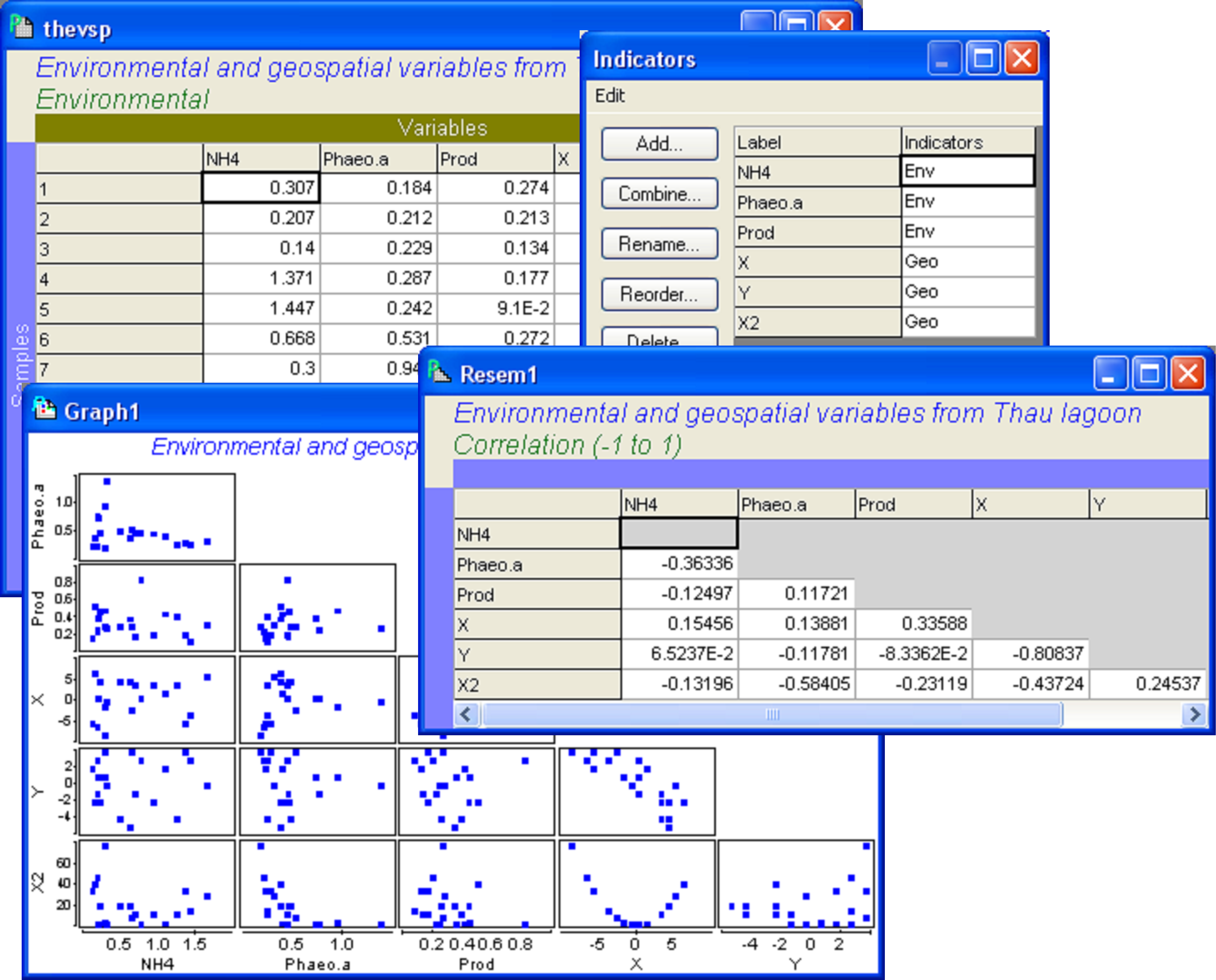
Fig. 4.19. Diagnostics examining predictor variables from the Thau lagoon.
The response variables, in this case, are concentrations of bacteria that contain no zeros and (after the log-transformation, which has already been done for these data) are quite well-behaved in their distributions (i.e., show fairly equal scatter throughout their range and are not heavily skewed). Thus, we can quite reasonably consider doing an analysis on the basis of the Euclidean distance measure. The variables are also in the same units of measurement and occur on similar scales, so no preliminary normalisation is needed here. Although normalisation of predictor variables is never required in DISTLM (and would make no difference to the results in any event), it is important to consider, when calculating Euclidean distances on the basis of a set of response variables, whether or not a prior normalisation is appropriate. For this, the usual considerations (such as the units of the variables and their relative scales) apply.
Calculate a Euclidean distance matrix from the thbac data sheet and then choose PERMANOVA+ > DISTLM > (Predictor variables worksheet: thevsp) & ($\checkmark$Group variables (indicator): Indicators) & (Selection Procedure •All specified) & (Selection Criterion •R^2) & (Num. permutations: 9999) & ($\checkmark$Do marginal tests), as shown in Fig. 4.20. Before clicking the ‘OK’ button, check out the order in which these sets of variables will be fitted by clicking on the ‘Select variables/groups…’ button. The order shown will be the order in which these groups were provided in the data file. In our case, however, it makes sense specifically to fit the ‘Geo’ set first, followed by the ‘Env’ set, as we are interested in testing the hypothesis of there being no relationship between the bacteria concentrations and the environmental variables, given the spatial variables. This can be done by highlighting Geo appearing inside the ‘Available:’ column and then clicking on the upward arrow to move it up to first in the list (Fig. 4.20).
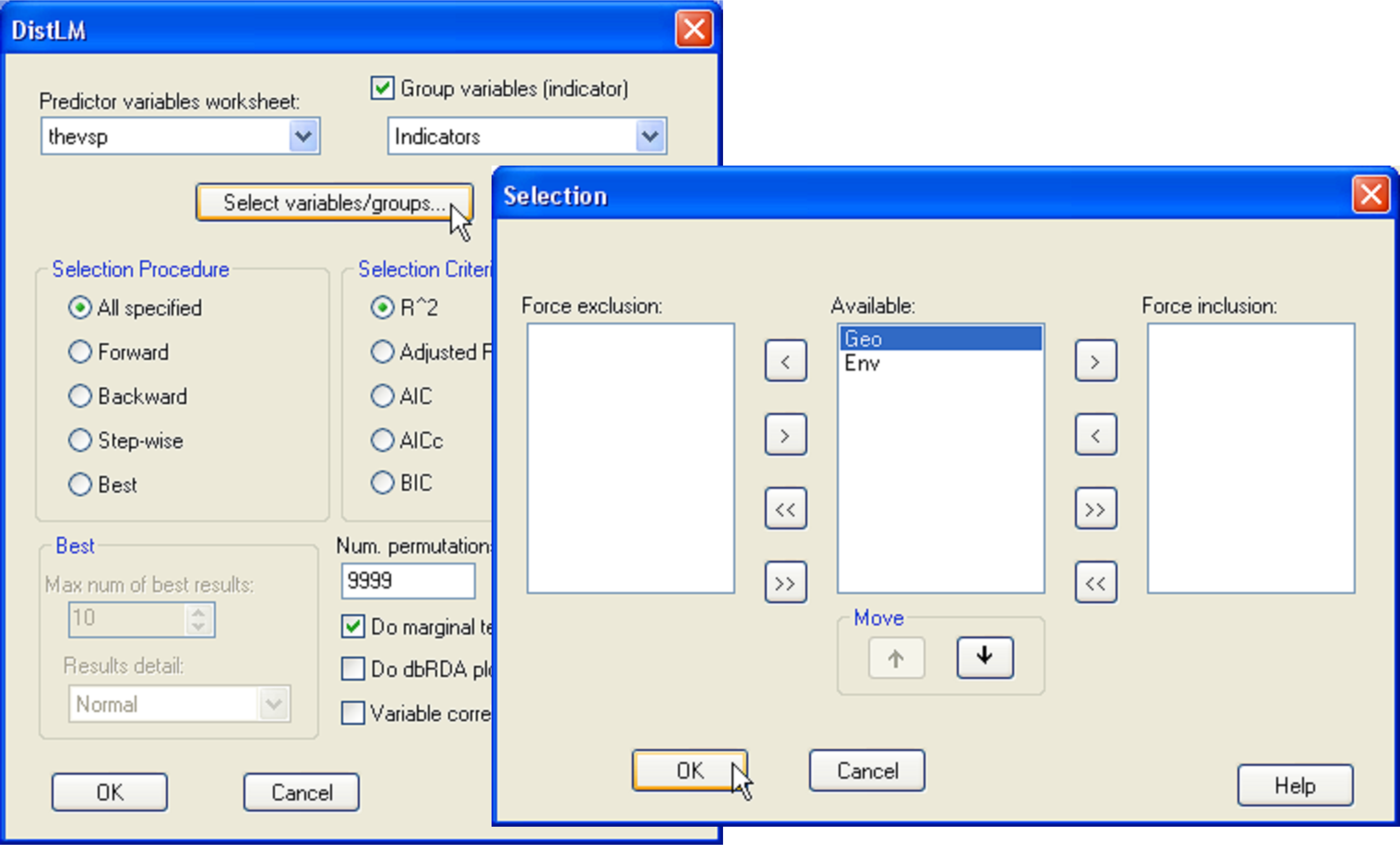 Fig. 4.20. DISTLM dialog for fitting sets of predictor variables in a particular order.
The file of results from this analysis is shown in Fig. 4.21. We can see that the three spatial variables alone accounted for 36.4% of the variation in the bacteria concentrations, while the environmental variables accounted for 45.0%. However, after fitting the spatial variables, the environmental variables explained an additional 18.5%, resulting in a total explained variation of 55%. This additional amount was not statistically significant, however, according to the sequential test (P = 0.16).
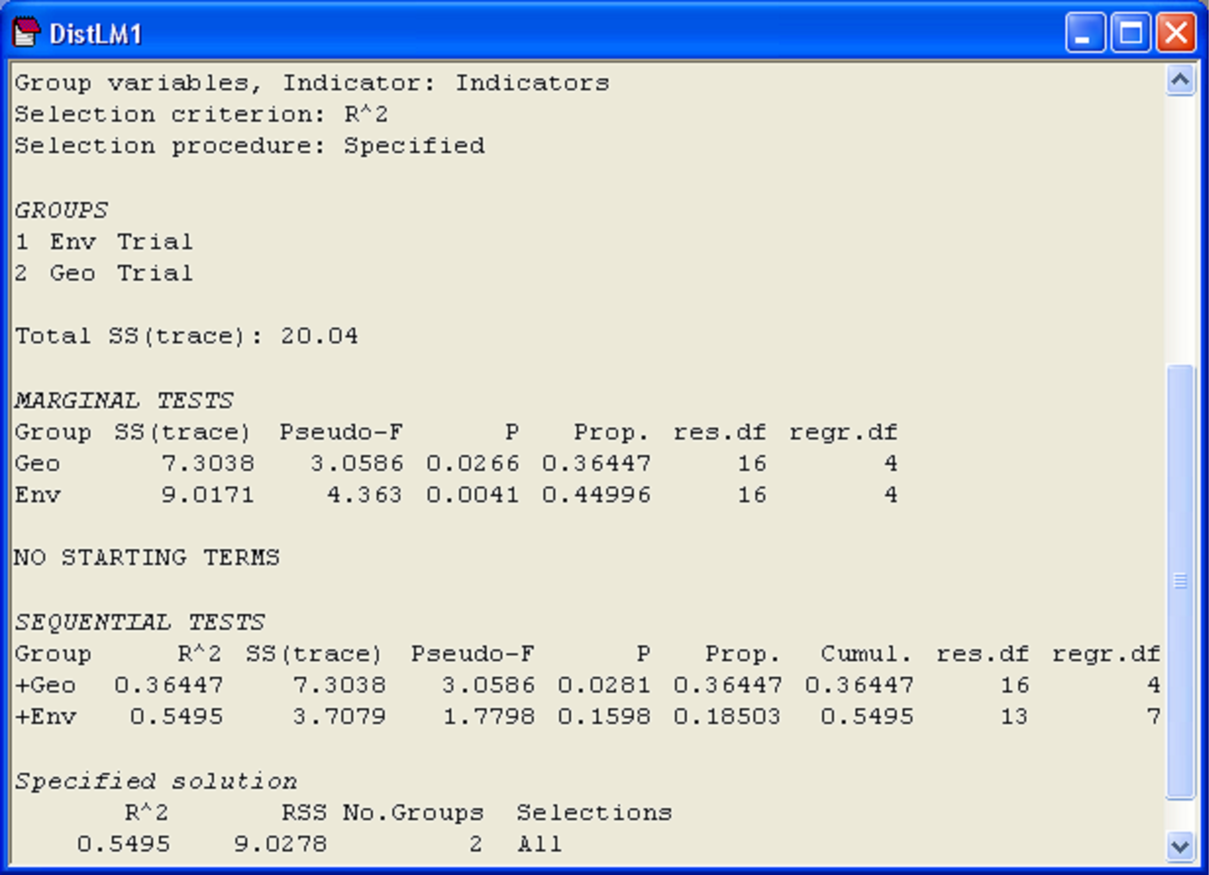 Fig. 4.21. Results of DISTLM fitting sets of predictor variables to bacteria concentrations from Thau lagoon.
Partitioning of multivariate data described by a resemblance matrix of choice in response to multiple sets of variables (as in Anderson & Gribble (1998) , for example, who partitioned temporal, spatial and environmental components) can be done in this manner, and the degree of overlap between individual sets can be readily determined by changing the order of fit of the variables, as desired. Keep in mind, however, that sets having different numbers of predictor variables will naturally have a different capability when it comes to explaining variation – a set with one variable would be expected naturally to explain less than a set with 5 variables, simply because it has fewer degrees of freedom. We have chosen in this example to use the simple R$^2$ criterion (both sets had 3 variables, so the percentage of variation explained could be directly compared), but an adjusted R$^2$, AIC, AIC$_c$ or BIC criterion could also be used, and these would (each in their own way) take into account different numbers of variables in the different sets93. Such an approach is directly analogous to examining components of variation derived from mean squares, rather than just looking at the raw partitioning of the sums of squares when comparing the relative importance of different sources of variation in a PERMANOVA model. In this example, we also had a specific hypothesis which dictated the order of the fit (the ‘Geo’ set first, followed by the ‘Env’ set), but in other situations, a different selection procedure (i.e., forward, backward, step-wise, best) might be more appropriate for the hypotheses or goals of the study.
93 Peres-Neto, Legendre, Dray et al. (2006) discussed the use of an adjusted R$^2$ criterion to perform a partitioning of multivariate response data in RDA and CCA models and to allow comparison of the sizes of portions explained by different sets of predictor variables.