1.25 Inference space and power
It is worthwhile pausing to consider how the above tests correspond to meaningful hypotheses for the mixed model. What is being examined by $F _ {Tr}$ is the extent to which the sum of squared fixed effects can be detected as being non-zero over and above the potential variability in these effects among blocks, i.e., over and above the interaction variability (if present). Thus, in a crossed mixed model like this, $F _ {Tr \times Bl}$ first provides a test of generality (i.e., do the effects of treatments vary significantly among blocks?), whereas the test of the main effect of treatments ($F _ {Tr}$) provides a test of the degree of consistency. In other words, even if there is variation in the effects of treatments (i.e. V(TrxBl) ≠ 0), are these consistent enough in their size and direction that an overall effect can be detected over and above this? Given the pattern shown in the MDS plot, it is not surprising to learn that, in this case, the main treatment effect is indeed discernible over and above the variation in its effects from block to block (P = 0.0037).
We can contrast these results with what would have happened if we had done this analysis but treated the blocks as fixed instead of random (Fig. 1.24). The consequence of this choice is a change to the EMS for the ‘Treatment’ term, which is now 1*V(Res) + 8*S(Tr) and therefore contains no component of variation for the interaction. As a consequence, the pseudo-F ratio for treatment main effects in this fully fixed model is constructed as $F _ {Tr} = MS _{Tr} / MS _ {Res}$ and, correspondingly, the denominator degrees of freedom for this test has increased from 3 to 8, the value of the pseudo-F ratio has changed from 4.67 to 8.08 and the P-value has decreased (cf. Figs. 1.23 & 1.24).
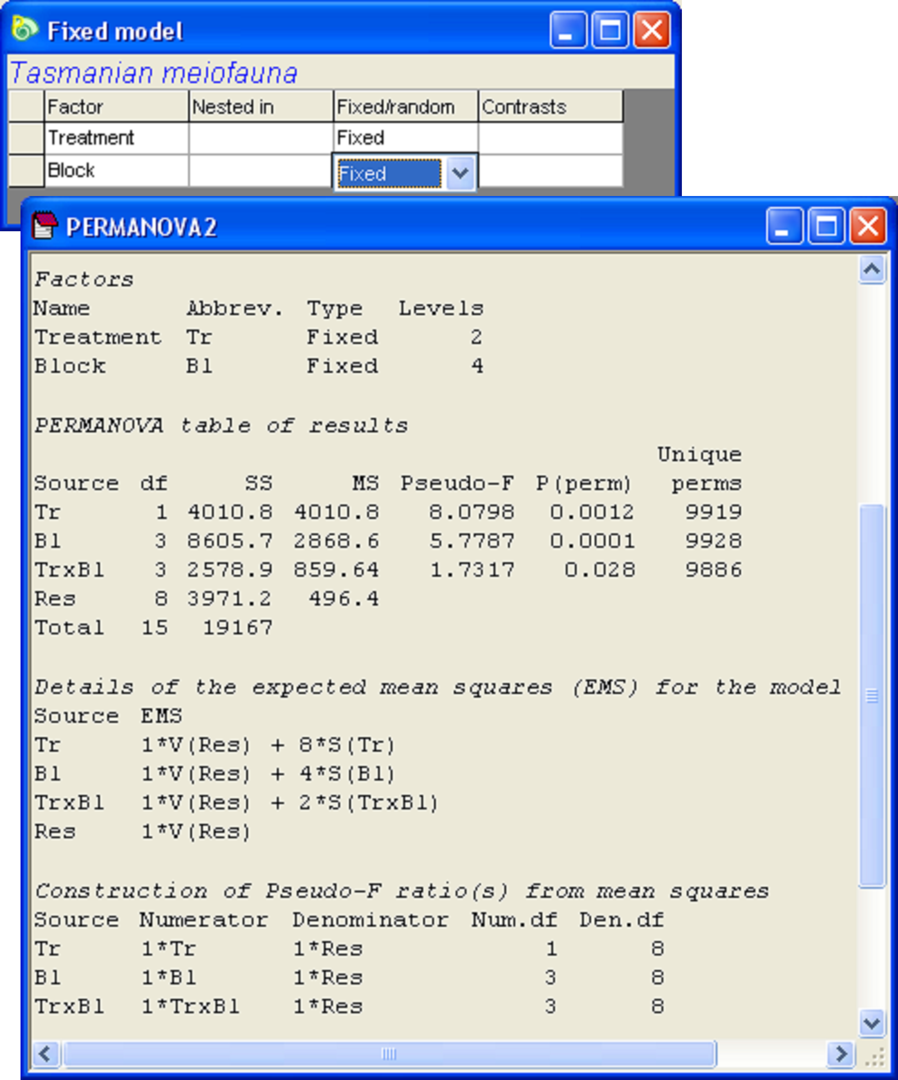 Fig. 1.24. Design file and analysis of Tasmanian meiofauna, treating the ‘Blocks’ as fixed.
On the face of it, we appear to have achieved a gain in power by using the fully fixed model in this case, as opposed to the mixed model that treated ‘Blocks’ as random. Power is the probability of rejecting the null hypothesis when it is false. When using a statistic like pseudo-F (or pseudo-t), power is generally increased by increases in the denominator degrees of freedom. Basically, the more information we have about a system, the easier it is to detect small effects. This choice of whether to treat a given factor as either fixed or random, however, doesn’t just affect the potential power of the test, it also rather dramatically affects the nature of our hypotheses and our inference space.
If we choose to treat ‘Blocks’ as random (Fig. 1.23), then: (i) the test of ‘TrxBl’ is a test of the generality of disturbance effects across blocks; (ii) the test of ‘Bl’ is a test of the spatial variability among blocks; and (iii) the test of ‘Tr’ is a test of the consistency in treatment effects, over and above the potential variability in its effects among blocks. Importantly, the inference space for each test refers to the population of possible blocks from which we could have sampled. In contrast, if we choose to treat ‘Blocks’ as fixed (Fig. 1.24), then: (i) the test of ‘TrxBl’ is a test of whether disturbance effects differ among those four particular blocks; (ii) the test of ‘Bl’ is a test of whether there are any differences among those four particular blocks; and (iii) the test of ‘Tr’ is a test of treatment effects, ignoring any potential variation in its effects among blocks. Also, the inference space for each of these tests in the fully fixed model refers only to those four blocks included in our experiment and no others.
In the end, it is up to the user to decide which hypotheses are the most relevant in a particular situation. The choice of whether to treat a given factor as fixed or random will dictate the EMS, the pseudo-F ratio, the extent of the inferences and the power of the tests in the model. Models with mixed and random effects will tend to have less power than models with only fixed effects. (Consider: in the context of the example, it would generally be easier to reject the null hypothesis that treatments have no effect whatsoever than it would be to reject the null hypothesis that treatments have no effect given some measured spatial variability in those effects.) However, random and mixed models can provide a much broader and therefore usually a more meaningful inference space (e.g., extending to the wider population of possible blocks across the sampled study area, and not just to those that were included in the experiment). Such models will therefore tend to correspond to much more logical and ecologically relevant hypotheses in many situations.
As we have seen, PERMANOVA employs direct multivariate analogues to the univariate results for the derivation of the EMS and construction of the pseudo-F ratio, so all of the well-known issues regarding logical inferences in experimental design that would occur for the univariate case (e.g., Cornfield & Tukey (1956) ; Underwood (1981) ; Hurlbert (1984) ; Underwood (1997) ) necessarily need to be considered for any multivariate analysis to be done by PERMANOVA as well.
As a final note regarding inference, the traditional randomization test is well known to be conditional on the order statistics of the data (e.g. Fisher (1935) ). In other words, the results (P-values) depend on the realised data values. This fact led Pitman ( Pitman (1937a) , Pitman (1937b) , Pitman (1937c) ) and Edgington (1995) to argue that the inferences from any test done using a randomization procedure can only extend to the actual data themselves, and can never extend to a wider population31. In a similar vein, Manly (1997) , section 7.6, stated that randomization tests must, by their very nature, only allow factors to be treated as fixed, because “Testing is conditional on the factor combinations used, irrespective of how these were chosen” (p. 142). PERMANOVA, however, uses permutation methods in order to obtain P-values, but it also (clearly) allows factors to be treated as random. How can this be?
Fisher (1935) considered the validity of a permutation test to be ensured by virtue of the a priori random allocation of treatments to individual units in an experiment. That is, random allocation before the experiment justifies randomization of labels to the data afterwards in order to create alternative possible outcomes we could have observed. However, we shall consider that a permutation test gains its validity more generally (such as, for example, in observational studies, where no a priori random allocation is possible), by virtue of (i) random sampling and (ii) the assumption of exchangeability under a true null hypothesis. As stated earlier (see the section Assumptions), PERMANOVA assumes only the exchangeability of appropriate units under a true null hypothesis. Random sampling of the levels of a random factor from a population of possible levels (like random sampling of individual samples), coupled with the assumption that “errors” (whether they be individual units or cells at a higher level in the design) are independent and identically distributed (“i.i.d.”) (e.g., Kempthorne (1952) ) ensures the validity of permutation tests for observational studies. For further discussion, see Kempthorne (1966) , Kempthorne & Doerfler (1969) and Draper, Hodges, Mallows et al. (1993) .
Thus, provided (i) the population from which levels have been chosen can be conceived of and articulated clearly, (ii) the exchangeability of levels can be asserted under a true null hypothesis and (iii) random sampling has been used, then the permutation test is valid for random factors, with an inference space that logically extends to that population. In section 7.3 of the more recent edition of Manly’s book ( Manly (2006) ), the validity of extending randomization procedures to all types of analysis of variance designs, including fixed and random factors, is also now acknowledged on the basis of this important notion of exchangeability ( Anderson & ter Braak (2003) ).
31 To be fair, Edgington (1995) also suggested that making such wider inferences using the normal-theory based tests was almost always just as much a “leap of faith” as it would be for a randomization test, due to the unlikely nature of the assumptions required by the former.