5.16 (Hunting spiders)
A study by van der Aart & Smeek-Enserink (1975) explored the relationships between two sets of variables: the abundances of hunting spiders (Lycosidae) obtained in pitfall traps and a suite of environmental variables for a series of sites across a dune meadow in the Netherlands. A subset of these data (p = 12 spider species, q = 6 environmental variables and N = 28 sites) are provided in the ‘Spiders’ folder of the ‘Examples add-on’ directory. Open up the files containing the spider data (hspi.pri) and the environmental variables (hspienv.pri) in PRIMER. Transform the spider data using an overall square-root transformation, then calculate a resemblance matrix using the chi-squared distance measure (D16). By using chi-squared distances as the basis for the analysis, we are placing a special focus on the composition of the spider assemblages in terms of proportional (root) abundances. Next, see the description of the environmental data by clicking on hspienv.pri and choosing Edit > Properties. The variables measured and included here are water content, bare sand, moss cover, light reflection, fallen twigs and herb cover, all on a log scale. A draftsman plot (including the choice $\checkmark$Correlations to worksheet) shows that no additional transformations are necessary. Also, the maximum correlation observed is between fallen twigs and light reflection (r = -0.87), so it is not really necessary to remove any of these variables. From the chi-squared resemblance matrix of square-root transformed spider data, choose PERMANOVA+ > CAP > (Analyse against •Variables in data worksheet: hspienv) & (Diagnostics $\checkmark$Do diagnostics) & (Do permutation test > Num. permutations: 9999), then click OK.
The results show that there were some very strong and significant correlations between the spider abundance data cloud (based on chi-squared distances) and the environmental variables (P = 0.0001). The first two canonical correlations are both greater than 0.90 (Fig. 5.24, $\delta _1$ = 0.9809, $\delta _2$ = 0.9256). Diagnostics revealed that the first m = 4 PCO axes (which together explained 92.7% of the total variability in the resemblance matrix) resulted in the smallest leave-one-out residual sum of squares, so there was no need to include more PCO axes in the analysis.
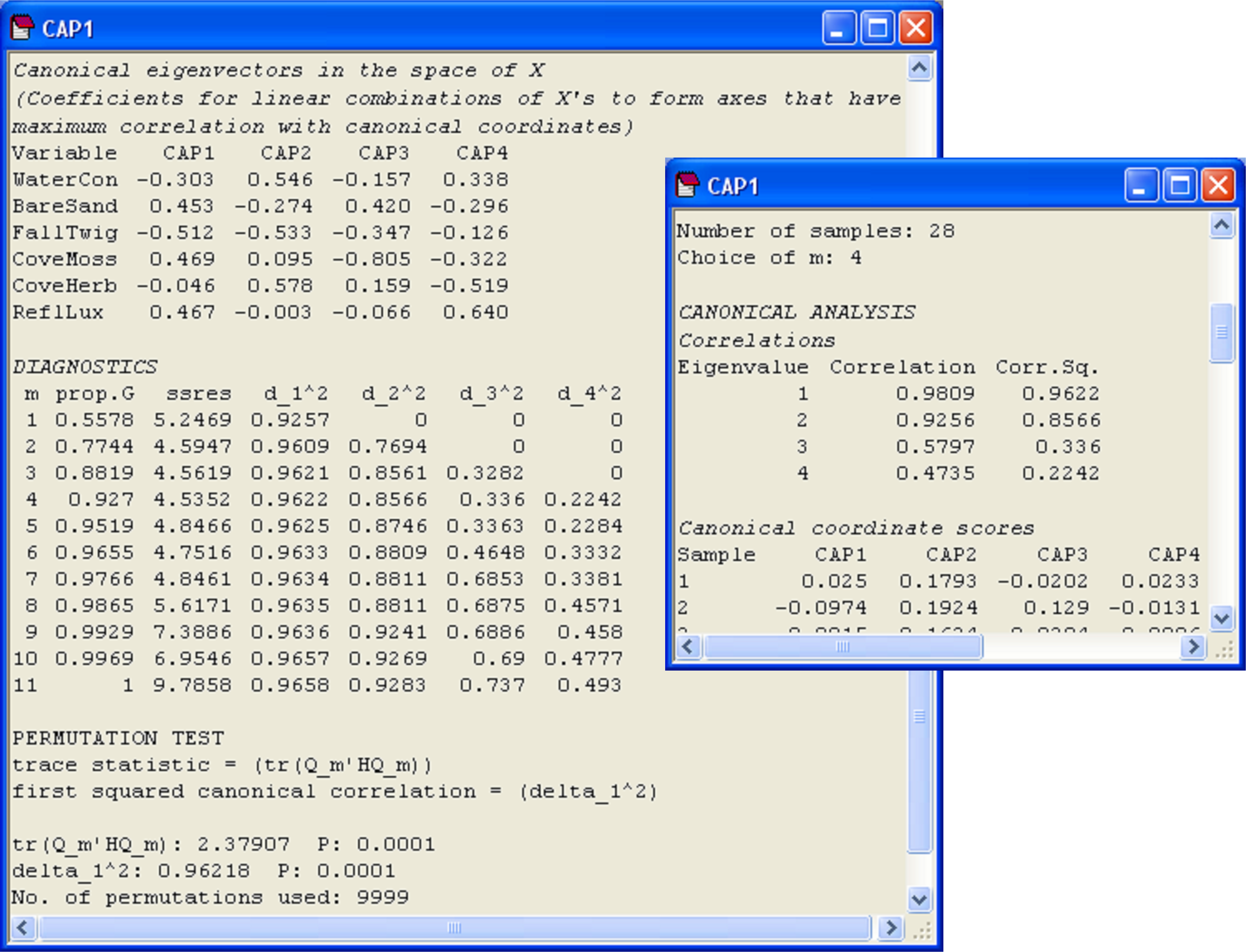 Fig. 5.24. Excerpts from the output file of the CAP analysis of the hunting spider data.
The CAP axes (‘Canonical coordinate scores’) given in the output file and also shown graphically in the plot are new variables (matrix C in Fig. 5.2) that are linear combinations of the PCO’s (based on the resemblance measure of choice) that have maximum correlation with the X’s. Also given in the output file are the weights, labeled ‘Canonical eigenvectors in the space of X’. These are the coefficients for linear combinations of the normalised X variables that will produce axes that have maximum correlation with the CAP axes. For example, the following linear combination of normalised X variables (produced using the weights given under ‘CAP1’ in the output file, Fig. 5.24):
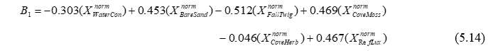
produces a new variable ($B_1$) that has maximum correlation with CAP axis 1 ($C_1$). Furthermore (and the reader is encouraged to verify this by hand, it is perfectly safe!), the Pearson correlation between these two variables ($B_1$ and $C_1$) is precisely the first canonical correlation of $\delta_1$ = 0.98. Similarly, the weights given for the normalised X variables for ‘CAP2’ will produce a second new variable ($B_2$), which is independent of (perpendicular to) the first variable ($B_1$) and has maximum correlation with CAP axis 2 ($C_2$), which is $\delta_2$ = 0.93, and so on. These eigenvector weights are also able to be seen visually on the CAP plot, as the default vector overlay for the X variables (Fig. 5.25).
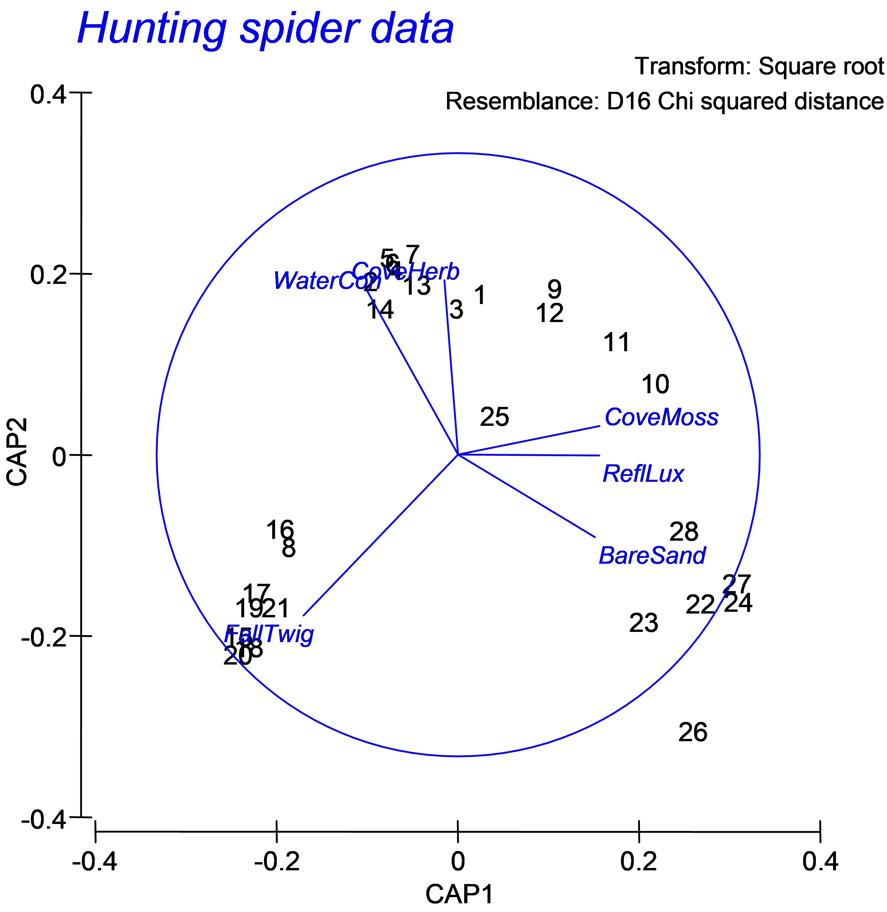 Fig. 5.25. CAP ordination plot relating hunting spiders to environmental variables.
One thing to be aware of here is that the CAP axes shown in the graphic and given in the output file as canonical coordinate scores are not a linear combination of the X variables, but of the PCO’s. Therefore, the default vector overlay shown in the CAP plot is not the same as what would be obtained by a direct projection of the X variables (as multiple partial correlations) onto these axes (i.e., using the ‘Multiple’ option as the correlation type in the ‘Configuration Plot’ dialog of Graph > Special). This contrasts with the dbRDA plot, where the relationships between the X variables and the dbRDA axes shown by the default vector overlay and the projected multiple partial correlations are indeed the same thing (see the section Vector overlays in dbRDA in chapter 4).
For the spiders dataset, we can see a fundamental shift in the structure of the assemblage that is strongly associated with the environmental variable of log percentage cover of fallen leaves and twigs (Fig. 5.25, see the samples numbered 16, 8, 17, 19, 21, 15, 20 and 18 at the bottom lower-left of the diagram and the associated vector labeled ‘FallTwig’). In addition, a gradient in community composition is evident among the other samples (stretching from the upper left to the lower right of the canonical plot), which is strongly related to log percentage of soil dry mass (‘WaterCon’) and log percentage cover of the herb layer (‘CoveHerb’) on the one hand, and log percentage cover of bare sand (‘BareSand’), moss cover (‘CoveMoss’) and light reflection (‘RefLux’) on the other.
Although the purpose here is to do little more than explore relationships, some clear patterns have emerged. Another vector overlay that can elucidate patterns, particularly for the spiders dataset, as we have just a few original species variables (p = 12), is to project the multiple partial correlations of these original variables (suitably transformed, in this case located in the worksheet named ‘Data1’) onto this plot (e.g., Fig. 5.26). Choose Graph > Special > (Vectors: •Worksheet variables: Data1 > Correlation type: Multiple). Certain species, such as Pardosa lugubris (‘Pardlugu’) and Trochosa terricola (‘Trocterr’) are associated with fallen leaves and twigs, while others, such as Arctosa perita (‘Arctperi’), Alopecosa fabrilis (‘Alopfabr’) and Alopecosa accentuata (‘Alopacce’), are associated with bare sand. This type of vector overlay, as outlined previously (see the section on Vector overlays in dbRDA), projects the (orthonormal) Y variables as multiple partial correlations onto the CAP axes. The cautions and caveats associated with interpreting vector overlays should be kept in mind for CAP, as for other ordination techniques in the PERMANOVA+ add-on package.
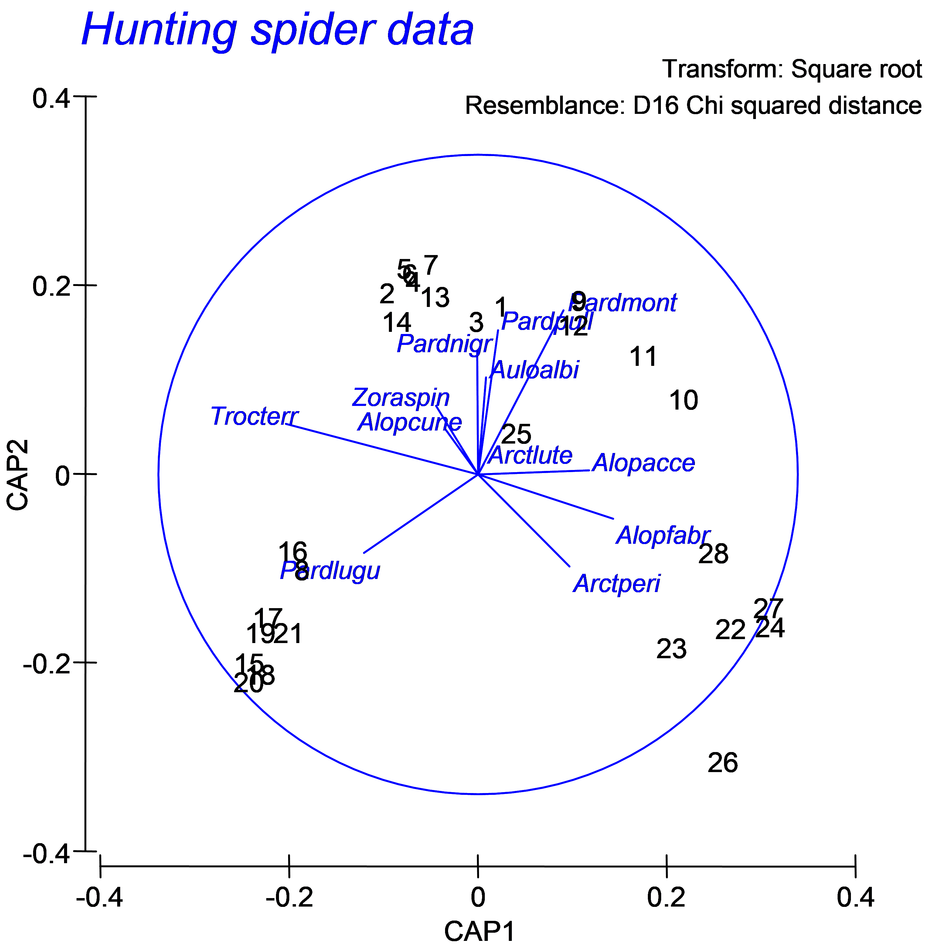 Fig. 5.26. CAP ordination plot relating hunting spiders to environmental variables, but with a vector overlay consisting of the multiple partial correlations of the original species variables (spider abundances, square-root transformed) with the canonical axes.